Project 2: Predicitng Customer Churn for a Mobile Phone Carrier
1. Overview
In this project, we will build a series of models to predict the probability of Customer Churn for a Mobile Phone Carrier.
In the first part, we will conduct Exploratory Data Analysis (EDA). Here the Synthetic Minority Oversampling Technique (SMOTE) method is employed to address the imbalanced classification problem. Then we will develop customer churn prediction models based on (1) Logistic Regression, (2) Decision Tree, (3) Random Forest, (4) AdaBoost, (5) Gradient Boosting Decision Trees (GBDT), and (6) Neural Network. With model hyperparameters optimized by GridSearchCV from sklearn package, the performance of each model is pretty good (measured by ROC-AUC, please see the table below).
| Model | ROC-AUC |
|---|---|
| Logistic Regression | 0.9219 |
| Decision Tree | 0.9138 |
| Random Forest | 0.9277 |
| Adaboost | 0.9373 |
| Gradient Boosting Decision Trees (GBDT) | 0.9260 |
| Neural Network | 0.9251 |
The Python Notebook containing the complete model development process and the data used in this project can be found at Google Drive.
2. Exploratory Data Analysis (EDA)
The dataset Google Drive of Customer Churn for a Mobile Phone Carrier is from SAS Financial Data Mining and Modeling (link). Since the computation was performed on Google Colab platform, we will first mount the Google Drive and load some useful packages.
from google.colab import drive
drive.mount('/content/drive')

import os
from datetime import datetime
import numpy as np
from scipy import stats
import pandas as pd
import statsmodels.api as sm
import statsmodels.formula.api as smf
import matplotlib.pyplot as plt
import seaborn as sns
import sklearn.metrics as metrics
from statsmodels.formula.api import ols
from sklearn.linear_model import LogisticRegression
from sklearn.preprocessing import StandardScaler
from sklearn import linear_model
from sklearn.svm import l1_min_c
from sklearn.model_selection import cross_val_score
import seaborn as sns
from sklearn.metrics import roc_auc_score
from sklearn.model_selection import GridSearchCV

from sklearn.tree import DecisionTreeClassifier
from sklearn.neural_network import MLPClassifier
from pylab import mpl

import pydotplus
from IPython.display import Image
import sklearn.tree as tree

from sklearn.model_selection import train_test_split
from imblearn.over_sampling import ADASYN
from imblearn.over_sampling import SMOTE
from imblearn.combine import SMOTETomek

from sklearn.preprocessing import MinMaxScaler
import sklearn.ensemble as ensemble
get_ipython().run_line_magic('matplotlib', 'inline')

pd.set_option('display.max_columns', None)

import warnings
warnings.filterwarnings('ignore')
# warnings.filterwarnings('default')
# pd.options.display.max_rows = 4000
By copying the dataset from Google Drive to the working directory and load it (see command and results below), we can see that the dataset is composed of 2484 rows and 19 variables. Each variable is examined carefully in the full script, here we will just examine one representative independent variable, duration, as well as the dependent variable churn.
2.1. Duration
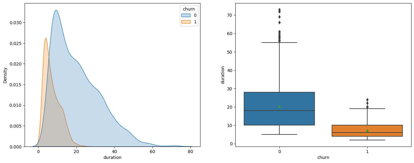
Variable ‘duration’ indicates the length of a customer relationship with the company. From the plots below, we can see that the duration for churned customers is much shorter, and this observation is also consistent with the F-test results that variable churn has a very large F value of 624.9 and very small p value of 3.36e-123.
fig = plt.figure(figsize=(16, 6))
ax1 = fig.add_subplot(1,2,1)
ax2 = fig.add_subplot(1,2,2)

sns.kdeplot(data=tel, x='duration', hue='churn', fill=True, ax=ax1)
sns.boxplot(x='churn', y='duration', data = tel, showmeans=True, ax=ax2)

tel.groupby('churn')[['duration']].describe().T
sm.stats.anova_lm(ols('duration ~ C(churn)',data=tel).fit())
| df | sum_sq | mean_sq | F | PR(>F) | |
|---|---|---|---|---|---|
| C(churn) | 1 | 73698 | 73698 | 624.9 | 3.36e-123 |
| Residual | 2482 | 292727 | 118 | NaN | NaN |
2.2. Churn
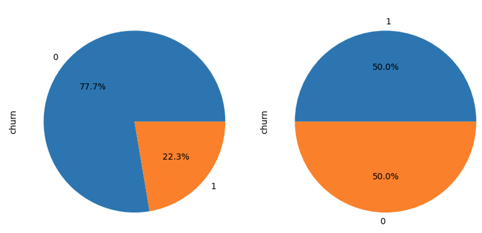
The dependent variable churn is examined below. In the first part of the code block, we examined itd distribution and found its distribution unbalanced. Then we split the dataset into training set and test set, and apply the Synthetic Minority Oversampling Technique (SMOTE) to the training set. The plots below shows the distribution of churn before (left) and after (right) applying SMOTE method. In the next section, we will use the rebalanced training set to develop model and the original test set to evaluate the model.
# Y - churn, 0 - False, 1 - True
tel.churn.value_counts().plot(kind = 'pie',autopct='%.1f%%')

# Split the dataset into train set and test set
train = tel.sample(frac = 0.8, random_state=76).copy()
test = tel[~tel.index.isin(train.index)].copy()
print(' Size of training set: %i \n Size of test set: %i' %(len(train), len(test)))

# Employ Synthetic Minority Oversampling Technique (SMOTE) for Imbalanced Classification
X_train = train.copy()
X_train.drop(['churn'], axis=1, inplace=True)
y_train = train.churn.copy()

X_test = test.copy()
X_test.drop(['churn'], axis=1, inplace=True)
y_test = test.churn.copy()

kos = SMOTE(random_state=0)
X_kos, y_kos = kos.fit_resample(X_train, y_train)
y_kos.value_counts().plot(kind = 'pie',autopct='%.1f%%')
3. Developing customer churn prediction model
This section is composed of four parts. In the first part, we will build model based on the Logistic Regression algorithm. In the second part, we will build model using Decision Tree. Then in part three Ensemble methods (i.e., Random Forest, AdaBoost, and GBDT) will be introduced. Finally in the fourth part, we will build a Neural Network-based model.
3.1. Logistic Regression
scaler = StandardScaler()
X_kos = scaler.fit_transform(X_kos)
X_test = scaler.transform(X_test)

cs = l1_min_c(X_kos, y_kos, loss='log') * np.logspace(-1, 7)
print("Computing regularization path ...")
start = datetime.now()
clf = linear_model.LogisticRegression(C=1.0, penalty='l1', tol=1e-6, max_iter=10000, solver='liblinear', verbose=1)
coefs_ = []
for c in cs:
    clf.set_params(C=c)
    clf.fit(X_kos, y_kos)
    coefs_.append(clf.coef_.ravel().copy())
print(' ')
print("This took ", datetime.now() - start)
coefs_ = np.array(coefs_)
plt.plot(np.log10(cs), coefs_)
ymin, ymax = plt.ylim()
plt.xlabel('log(C)')
plt.ylabel('Coefficients')
plt.title('Logistic Regression Path')
plt.axis('tight')
plt.show()

cs = l1_min_c(X_kos, y_kos, loss='log') * np.logspace(-1, 7)
k_scores = []
clf = linear_model.LogisticRegression(penalty='l1')
clf = linear_model.LogisticRegression(penalty='l1', tol=1e-4, max_iter=10000, solver='liblinear', verbose=1)
#http://scikit-learn.org/stable/modules/model_evaluation.html
for c in cs:
    clf.set_params(C=c)
    scores = cross_val_score(clf, X_kos, y_kos, cv=4, scoring='roc_auc')
    k_scores.append([c,scores.mean(),scores.std()])

data=pd.DataFrame(k_scores) #convert dict to dataframe
fig = plt.figure()
ax1 = fig.add_subplot(111)
ax1.plot(np.log10(data[0]), data[1],'b')
ax1.set_ylabel('Mean ROC (Blue)')
ax1.set_xlabel('log10(cs)')
ax2 = ax1.twinx()
ax2.plot(np.log10(data[0]), data[2],'r')
ax2.set_ylabel('Std ROC Index (Red)')
ax2.axline([-1.1, 0], [-1.1, 0.04])
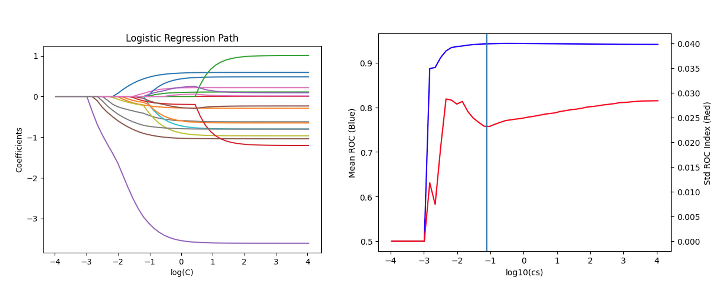
The code and plots above shows the development of a multivariate logistic regression with L1 regularization. We compute the regularization path and visualize the mean and standard derivation of ROC vs inverse of regularization strength C. The figure shows that optimal value of C should be near exp(-1.1).

clf = linear_model.LogisticRegression(C=np.exp(-1.1), penalty='l1',max_iter=10000, solver='liblinear', verbose=1)
clf.fit(X_kos, y_kos)

y_kos_pred = clf.predict(X_kos)
y_kos_proba = clf.predict_proba(X_kos)[:, 1]
y_test_pred = clf.predict(X_test)
y_test_proba = clf.predict_proba(X_test)[:, 1]

print('confusion_matrix')
print(metrics.confusion_matrix(y_test, y_test_pred))
print('classification_report')
print(metrics.classification_report(y_test, y_test_pred))

fpr_train, tpr_train, th_train = metrics.roc_curve(y_kos, y_kos_proba)
fpr_test, tpr_test, th_test = metrics.roc_curve(y_test, y_test_proba)
plt.figure(figsize=[6,6])
plt.plot(fpr_train, tpr_train, 'r-', label='train_data')
plt.plot(fpr_test, tpr_test, 'b--', label='test_data')
plt.title('ROC curve')
plt.axline([0, 0], [1, 1])
plt.xlim([-0.02, 1])
plt.ylim([0, 1.02])
plt.xlabel('FPR')
plt.ylabel('TPR')
plt.legend()

test['prediction'] = (y_test_proba > 0.5).astype('int')
acc = sum(test['prediction'] == test['churn']) /float(len(test))
print('The accurancy is %.4f' %acc)

print('AUC = %.4f' %metrics.auc(fpr_test, tpr_test))
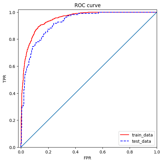
Then we can use the code above to generate model predictions and plotting the corresponding ROC curve. From ROC curve, we can see that for both the training set (with SMOTE) and test set (without SMOTE), the Logistic Regression model gives very good result, and this observation is further confirmed by AUC = 0.9219.
3.2. Decision Tree
param_grid = {
    'criterion':['entropy','gini'],
    'max_depth':[4, 8, 12, 16],
    'min_samples_split':[100, 120, 140, 160]
}

dtclf = tree.DecisionTreeClassifier(random_state=92)
clfcv = GridSearchCV(dtclf, param_grid=param_grid, scoring='roc_auc' ,cv=4, n_jobs=-1, verbose=2)
clfcv.fit(X_kos, y_kos)

dtclf = tree.DecisionTreeClassifier(criterion='gini', max_depth=8, min_samples_split=140, random_state=92)
dtclf.fit(X_kos, y_kos)

dot_data = tree.export_graphviz(
    dtclf,
    out_file=None,
    feature_names=X_train.columns,
    max_depth=2,
    class_names=['0','1'],
    filled=True
)
graph = pydotplus.graph_from_dot_data(dot_data)
Image(graph.create_png())
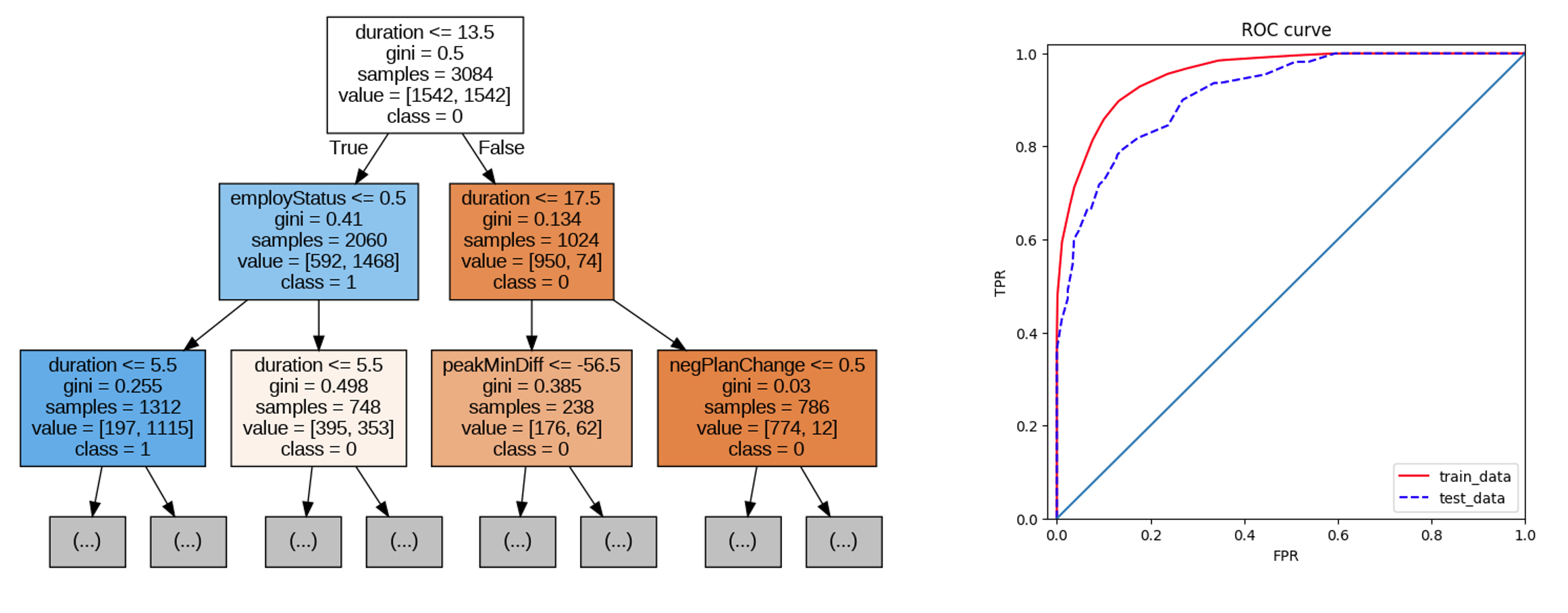
The decision tree based model is shown in the code and figure above. From the visualization of the tree on the left plot, we can see that variable duration is indeed very important for predicting the customer churn. The model has a pretty nice ROC curve and its AUC is quite high too (i.e., 0.9138).
3.3. Ensemble methods
# Random Forest
param_grid = {
'max_depth':[10, 100, 1000],
'max_features':[0.001, 0.01, 0.1], #number of features to consider when looking for the best split
'min_samples_split':[2, 4],
'n_estimators':[2000, 4000, 8000] #number of trees in the forest
}
rfc = ensemble.RandomForestClassifier()
rfccv = GridSearchCV(estimator=rfc, param_grid=param_grid, scoring='roc_auc', cv=4, n_jobs=-1, verbose=5)
rfccv.fit(X_kos, y_kos)

# Adaboost
param_grid = {
'learning_rate':[0.3, 1, 3],
'n_estimators':[200, 400, 800] #number of trees
}
abc = ensemble.AdaBoostClassifier(algorithm='SAMME')
abccv = GridSearchCV(estimator=abc, param_grid=param_grid, scoring='roc_auc', cv=4,n_jobs=-1, verbose=10)
abccv.fit(X_kos, y_kos)

# Gradient Boosting Decision Trees (GBDT)
param_grid = {
'learning_rate':[0.4, 0.8, 1.2],
'max_depth':[5, 10, 15],
'n_estimators':[30, 50, 70],
}

gbc = ensemble.GradientBoostingClassifier(random_state=12)
gbccv = GridSearchCV(estimator=gbc, param_grid=param_grid, scoring='roc_auc', cv=4,n_jobs=-1, verbose=10)
gbccv.fit(X_kos, y_kos)
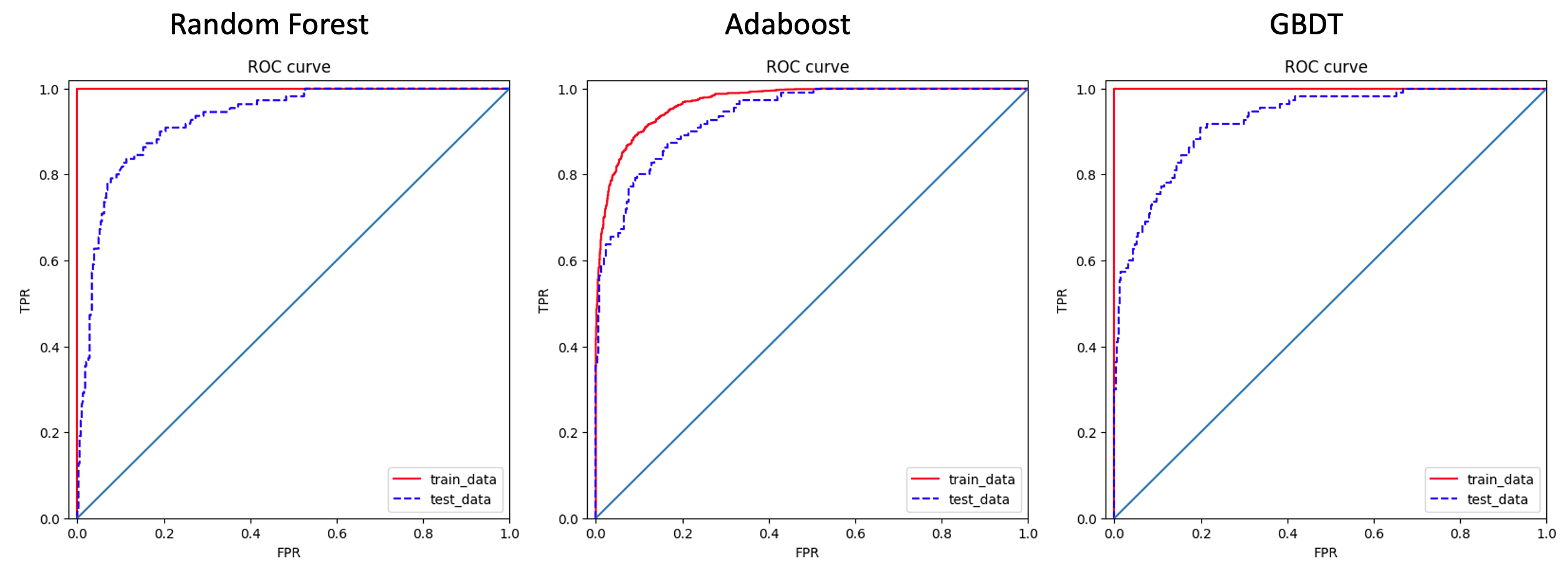
Three popular ensemble methods (i.e., Random Forest, AdaBoost, GBDT) are also applied to develop customer churn prediction models. Part of the code are shown above, together with their ROC curves. As we expected, all three method have very good ROC performance, and their AUC values are 0.9277 (Random Forest), 0.9373 (AdaBoost), 0.9260 (GBDT).
3.4. Neural Network
# Standardize features
scaler = StandardScaler()
X_kos_scaled = scaler.fit_transform(X_kos)
X_test_scaled = scaler.transform(X_test)

param_grid={
'alpha':[0.5, 1, 2],
'hidden_layer_sizes':[(100,100), (200,200), (300,300), (400,400)],
}

mlp=MLPClassifier()
gcv=GridSearchCV(estimator=mlp,param_grid=param_grid, scoring='roc_auc', cv=4, n_jobs=-1, verbose=10)
gcv.fit(X_kos_scaled,y_kos)
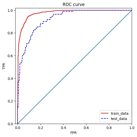
Finally, we use the MLPClassifier module from sklearn to develop a very simple neural network for customer churn prediction. From the ROC curve shown above, we can see that the model also gives very good results, and the corresponding AUC is 0.9251.
4. Conclusions
In this work, I have developed a series of models to predict customer churn for a mobile phone carrier. Among all the methods I tried, I would recommend AdaBoost if model interpretability is not required, because it is fast, robust, and very accurate. On the other hand, if “black box” model is not acceptable, then I would recommend Multivariate logistic regression with L1 regularization, because it is explainable and with careful hyperparameter tuning, very accurate prediction too.