Project 4: Image Classification and Explainable Artificial Intelligence
1. Project Overview
In this project, we will build a model for image classification and understand how it works.
In the first part, we will develop a convolutional neural network (CNN) model for food image classification. We will also apply t-distributed Stochastic Neighbor Embedding (t-SNE) technique on the output of different layers to visualize learned visual representations of the CNN model.
In order to understand how the model works, we will employ four popular Explainable AI approaches in the second part, including (1) Saliency map, (2) Smooth gradient, (3) Lime package, and (4) Integrated gradients.
The Python Notebook containing the complete model development process and the data used in this project can be found at Google Drive.
2. CNN model for food images classification
2.1. Dataset
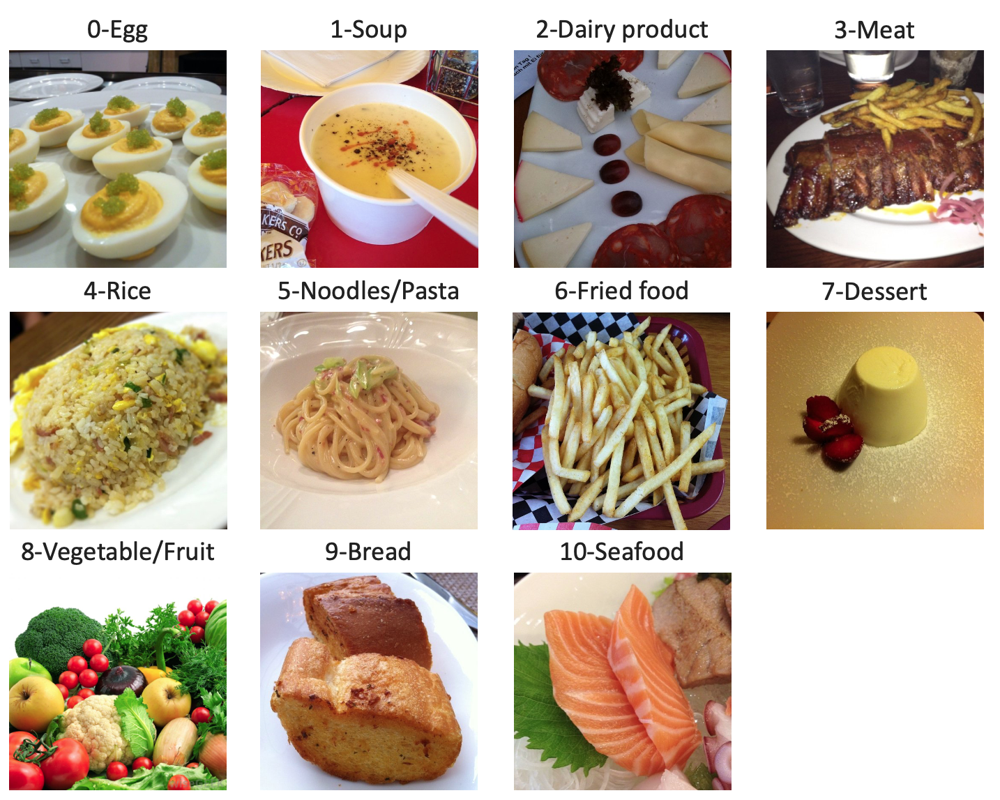
The Food-11 image dataset used in this project is originally from École Spéciale de Lausanne. This dataset contains 16643 food images grouped in 11 major food categories, including egg, soup, dairy product, meat, rice, noodles/pasta, fried food, dessert, vegetable/fruit, bread, and seafood, as shown in the picture below.
2.2. CNN Model
# Model definition
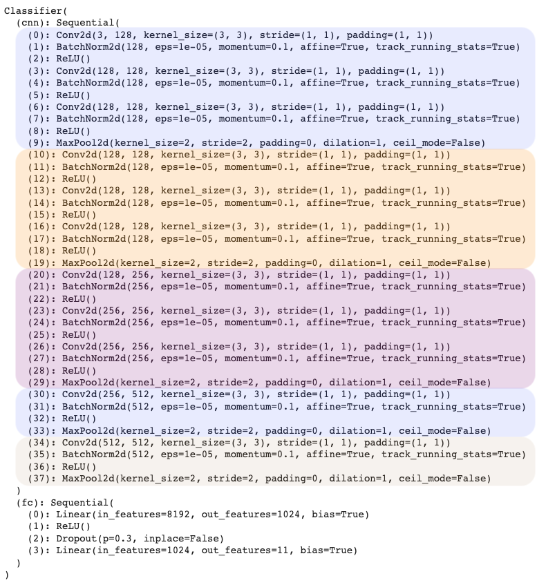
class Classifier(nn.Module):
def __init__(self):
super(Classifier, self).__init__()
def building_block(indim, outdim):
return [
nn.Conv2d(indim, outdim, 3, 1, 1),
nn.BatchNorm2d(outdim),
nn.ReLU(),
]
def stack_blocks(indim, outdim, block_num):
layers = building_block(indim, outdim)
for i in range(block_num - 1):
layers += building_block(outdim, outdim)
layers.append(nn.MaxPool2d(2, 2, 0))
return layers
cnn_list = []
cnn_list += stack_blocks(3, 128, 3)
cnn_list += stack_blocks(128, 128, 3)
cnn_list += stack_blocks(128, 256, 3)
cnn_list += stack_blocks(256, 512, 1)
cnn_list += stack_blocks(512, 512, 1)
self.cnn = nn.Sequential( * cnn_list)
dnn_list = [
nn.Linear(512 * 4 * 4, 1024),
nn.ReLU(),
nn.Dropout(p = 0.3),
nn.Linear(1024, 11),
]
self.fc = nn.Sequential( * dnn_list)
def forward(self, x):
out = self.cnn(x)
out = out.reshape(out.size()[0], -1)
return self.fc(out)
The code block above shows the architecture of the convolutional neural network (CNN) model used in this project. An useful reference of this architecture can be found here.
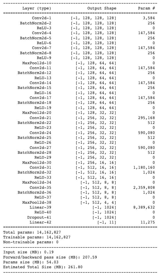
The picture below shows the model structure, with each block highlighted in different colors. In particular, the model is composed of a CNN part followed by a fully connected part. The CNN part contains five stacked blocks: the first three blocks are similar to each other (3*(Conv2d-BatchNorm2d-ReLU)+MaxPool2d) and the last two blocks are similar to each other (1*(Conv2d-BatchNorm2d-ReLU)+ MaxPool2d). Batch Normalization ref is an useful technique for model optimization. By adding it to the model, we are able to train the model faster and more stable. The model summary is shown in the second picture below, the total number of parameters is 14.2M.
During model training, we apply image transformations ref (see code block below) to modify the image data so that more diversified inputs are given to the model in each epoch, in order to improve mode performance and prevent overfitting.
train_tfm = transforms.Compose([
    transforms.Resize(size=(128, 128)),
    transforms.RandomHorizontalFlip(),
    transforms.RandomRotation(15),
    transforms.ToTensor(),
])
test_tfm = transforms.Compose([
    transforms.Resize(size=(128, 128)),
    transforms.ToTensor(),
])
The code block below shows the training and test part of the model.
# Initialize trackers
stale = 0
best_acc = 0

for epoch in range(n_epochs):

    # ---------- Training ----------
    model_ft.train() # Make sure the model is in train mode before training
    train_loss = []
    train_accs = []
    since = time.time() # Starting time of each epoch
    for batch in tqdm(train_loader):
        imgs, labels = batch # A batch consists of image data and corresponding labels.
        logits = model_ft(imgs.to(device))
        loss = criterion(logits, labels.to(device)) # Calculate the cross-entropy loss. don't need to apply softmax before computing cross-entropy as it is done automatically
        optimizer.zero_grad() # Gradients stored in the parameters in the previous step should be cleared out first.
        loss.backward() # Compute the gradients for parameters
        grad_norm = nn.utils.clip_grad_norm_(model_ft.parameters(), max_norm=10) # Clip the gradient norms for stable training.
        optimizer.step() # Update the parameters with computed gradients
        acc = (logits.argmax(dim=-1) == labels.to(device)).float().mean()
        train_loss.append(loss.item())
        train_accs.append(acc)

    train_loss = sum(train_loss) / len(train_loss)
    train_acc = sum(train_accs) / len(train_accs)
    print(f"[ Train | {epoch + 1:03d}/{n_epochs:03d} ] loss = {train_loss:.5f}, acc = {train_acc:.5f}")

    # ---------- Validation ----------
    model_ft.eval() # Make sure the model is in eval mode so that some modules like dropout are disabled and work normally
    valid_loss = []
    valid_accs = []
    for batch in tqdm(valid_loader):
        imgs, labels = batch
        with torch.no_grad(): # Using torch.no_grad() accelerates the forward process because we don't need gradient in validation.
            logits = model_ft(imgs.to(device))
        loss = criterion(logits, labels.to(device)) # Still need to compute loss but not gradient.
        acc = (logits.argmax(dim=-1) == labels.to(device)).float().mean()
        valid_loss.append(loss.item())
        valid_accs.append(acc)
    valid_loss = sum(valid_loss) / len(valid_loss)
    valid_acc = sum(valid_accs) / len(valid_accs)
    print(f"[ Valid | {epoch + 1:03d}/{n_epochs:03d} ] loss = {valid_loss:.5f}, acc = {valid_acc:.5f}")

    # update logs
    if valid_acc > best_acc:
        with open(f"./P4-log.txt","a") as log:
            print(f"[ Valid | {epoch + 1:03d}/{n_epochs:03d} ] loss = {valid_loss:.5f}, acc = {valid_acc:.5f} -> best")
            log.write(f"[ Valid | {epoch + 1:03d}/{n_epochs:03d} ] loss = {valid_loss:.5f}, acc = {valid_acc:.5f} -> best")
    else:
        with open(f"./P4-log.txt","a") as log:
            print(f"[ Valid | {epoch + 1:03d}/{n_epochs:03d} ] loss = {valid_loss:.5f}, acc = {valid_acc:.5f}")
            log.write(f"[ Valid | {epoch + 1:03d}/{n_epochs:03d} ] loss = {valid_loss:.5f}, acc = {valid_acc:.5f}")

    # save models
    if valid_acc > best_acc:
        print(f"Best model found at epoch {epoch}, saving model")
        torch.save(model_ft.state_dict(), f"P4-best.ckpt")
        %cd /content
        best_acc = valid_acc
        stale = 0
    else:
        stale += 1
        if stale > patience:
            print(f"No improvment {patience} consecutive epochs, early stopping")
            break

    time_elapsed = time.time() - since
    print('Training complete in {:.0f}m {:.0f}s'.format(time_elapsed // 60, time_elapsed % 60))
    print('Best val Acc: {:4f}'.format(best_acc))

# ---------- Test ----------
# Construct test datasets.
test_set = FoodDataset("./food/test", tfm=test_tfm)
test_loader = DataLoader(test_set, batch_size=batch_size, shuffle=False, num_workers=0, pin_memory=True)

model_best = model_ft.to(device)
!cp /content/drive/MyDrive/210-Projects/410_Image_Classification/P4-best.ckpt P4-best.ckpt
model_best.load_state_dict(torch.load(f"P4-best.ckpt"))
model_best.eval()

test_loss = []
test_accs = []
for batch in tqdm(test_loader):
    imgs, labels = batch
    with torch.no_grad():
        logits = model_ft(imgs.to(device))
    loss = criterion(logits, labels.to(device))
    acc = (logits.argmax(dim=-1) == labels.to(device)).float().mean()
    test_loss.append(loss.item())
    test_accs.append(acc)
test_loss = sum(test_loss) / len(test_loss)
test_accs = sum(test_accs) / len(test_accs)
print(f" Test loss = {test_loss:.5f}, acc = {test_accs:.5f}")
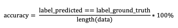
In this project, we use accuracy to evaluate model performance.
device = "cuda" if torch.cuda.is_available() else "cpu" # "cuda" only when GPUs are available.
batch_size = 64 # The number of batch size.
n_epochs = 1000 # The number of training epochs.
patience = 50 # If no improvement in patience epochs, early stop.
criterion = nn.CrossEntropyLoss() # Classification task use cross-entropy
feature_extract = False # Flag for feature extracting. When False finetune the whole model, when True only update the reshaped layer params
By using the settings shown above, we are able to achieve 99% accuracy on training set and 91% accuracy on test set.
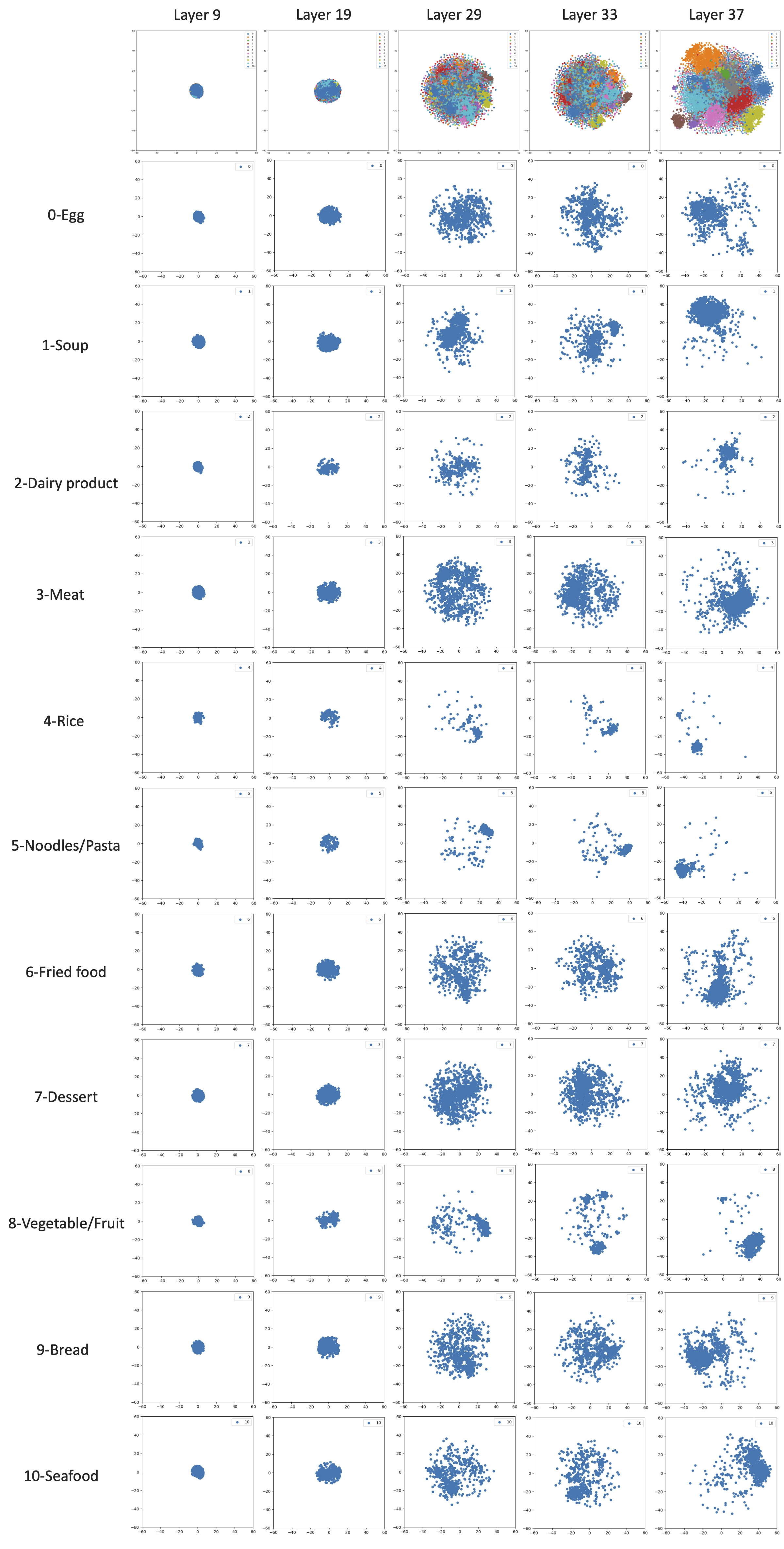
2.3. Layer output visualized by t-SNE
In this section, we will use the t-distributed stochastic neighbor embedding (t-SNE) technique to visualize the output of different layers of the CNN model developed in the previous section. The selected layers are circled blue in the picture below, which corresponding to the last layer of each block.

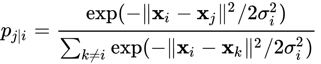
t-SNE is a useful method for high-dimensional data visualization wiki. In brief, for a set of high-dimensional objects x_1, x_2, …, x_N, t-SNE first computes
and p_ij = (p_j|i + p_i|j)/2N.
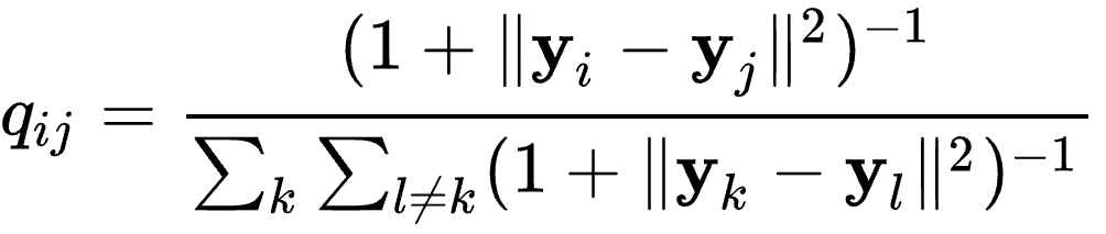
Then t-SNE aims to learn a d-dimensional map y_1, y_2, …, y_N (with d=2 in this section) that reflects the similarities p_ij as well as possible. To this end, it measures similarities q_ij by
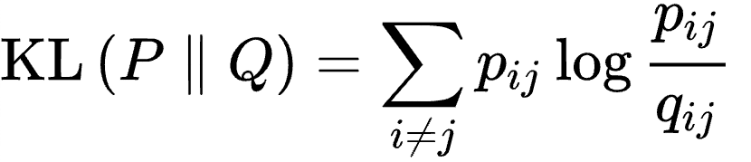
and the locations of the points y_i are determined by minimizing the Kullback–Leibler divergence of the distribution P from the distribution Q using gradient descent:
# Extract the representations for the specific layer of model
index = 38 # 10, 20, 30, 34, 38
features = []
labels = []
for batch in tqdm(tsne_loader):
    imgs, lbls = batch
    with torch.no_grad():
        logits = model_ft.cnn[:index](imgs.to(device))
        logits = logits.view(logits.size()[0], -1)
    labels.extend(lbls.cpu().numpy())
    logits = np.squeeze(logits.cpu().numpy())
    features.extend(logits)
features = np.array(features)
colors_per_class = cm.rainbow(np.linspace(0, 1, 11))
# Apply t-SNE to the features
features_tsne = TSNE(n_components=2, init='pca', random_state=42).fit_transform(features)
# Plot the t-SNE visualization
plt.figure(figsize=(10, 10))
for label in np.unique(labels):
    plt.scatter(features_tsne[labels == label, 0], features_tsne[labels == label, 1], alpha=0.75, label=label, s=50)
plt.legend()
plt.xlim(-60, 60)
plt.ylim(-60, 60)
plt.show()
# Plot the t-SNE visualization of each label
for label in np.unique(labels):
    plt.figure(figsize=(5, 5))
    plt.scatter(features_tsne[labels == label, 0], features_tsne[labels == label, 1], label=label, s=25)
    plt.xlim(-60, 60)
    plt.ylim(-60, 60)
    plt.legend()
    plt.show()
With the help of sklearn’s Manifold package, the realization of t-SNE is quite straightforward (see code block above), and the results are shown in the picture below. As we move from bottom layers to mid layers and top layers (Layer 9 -> Layer 19 -> Layer 29 -> Layer 33 -> Layer 37), visual representation of each class gradually separate apart.
3. Understanding CNN model with Explainable AI techniques
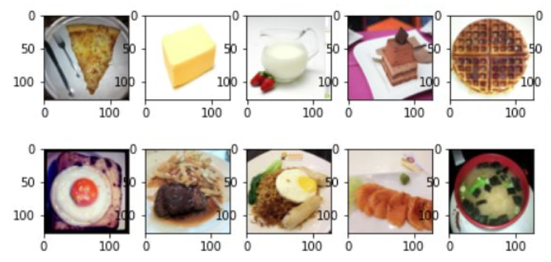
In order to understand how the CNN model works, we will employ four popular Explainable AI approaches in this part, including Saliency map, Smooth gradient, Lime package, and Integrated gradients. We will apply these methods to the 10 pictures below.
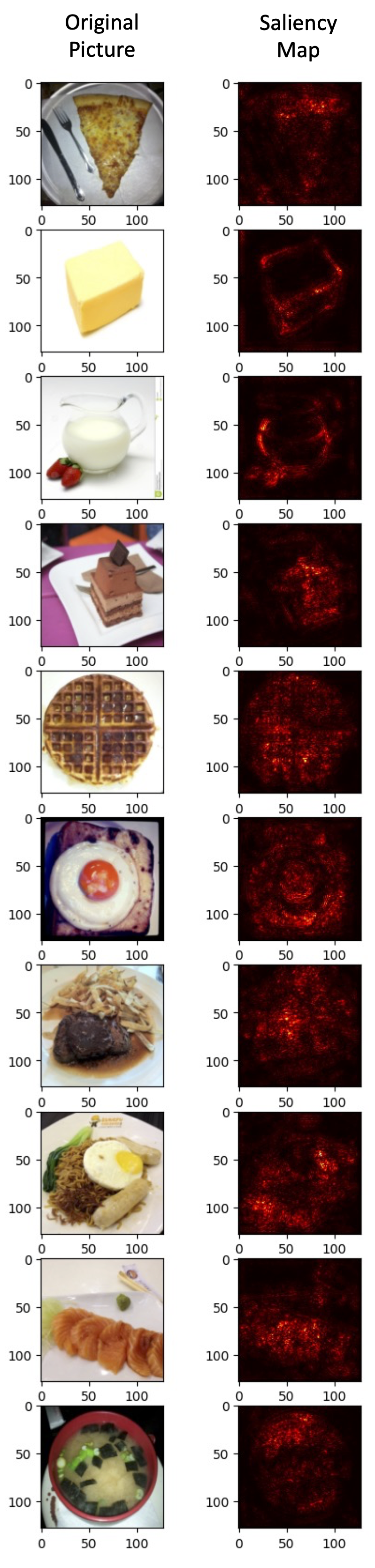
3.1. Saliency Map
The first method we will apply is the Saliency Map method Ref. This method aims to measure the importance of each pixel in the picture by perturbing the pixel value and calculating the partial differential value of loss to the modified picture. The output is a heatmap that highlight pixels of the input image that contribute the most in the classification task. In this way, we can visualize it to determine which part of the image contribute the most to the model’s judgment.
# Saliency Map
def normalize(image):
  return (image - image.min()) / (image.max() - image.min())

def compute_saliency_maps(x, y, model):
  model.eval()
  x = x.cuda()
  x.requires_grad_()   # we want the gradient of the input x
  y_pred = model(x)
  loss_func = torch.nn.CrossEntropyLoss()
  loss = loss_func(y_pred, y.cuda())
  loss.backward()
  saliencies, _ = torch.max(x.grad.data.abs().detach().cpu(),dim=1)
  saliencies = torch.stack([normalize(item) for item in saliencies]) # We need to normalize each image, because their gradients might vary in scale
  return saliencies

saliencies = compute_saliency_maps(images, labels, model_ft)

fig, axs = plt.subplots(len(img_indices), 2, figsize=(5, 20))
for row, target in enumerate([images, saliencies]):
  for column, img in enumerate(target):
    if row==0:
      # Pytorch:    each dimension of image tensor is (channels, height, width)
      # Matplotlib: each dimension of image tensor is (height, width, channels)
      axs[column][row].imshow(img.permute(1, 2, 0).numpy())
    else:
      axs[column][row].imshow(img.numpy(), cmap=plt.cm.hot)
plt.show()
plt.close()
The code blocks above shows the realization of Saliency Map, with the results shown below. From this figure, we can see that the Saliency Map method is able to show which pixels are critical for CNN model to understand the picture.
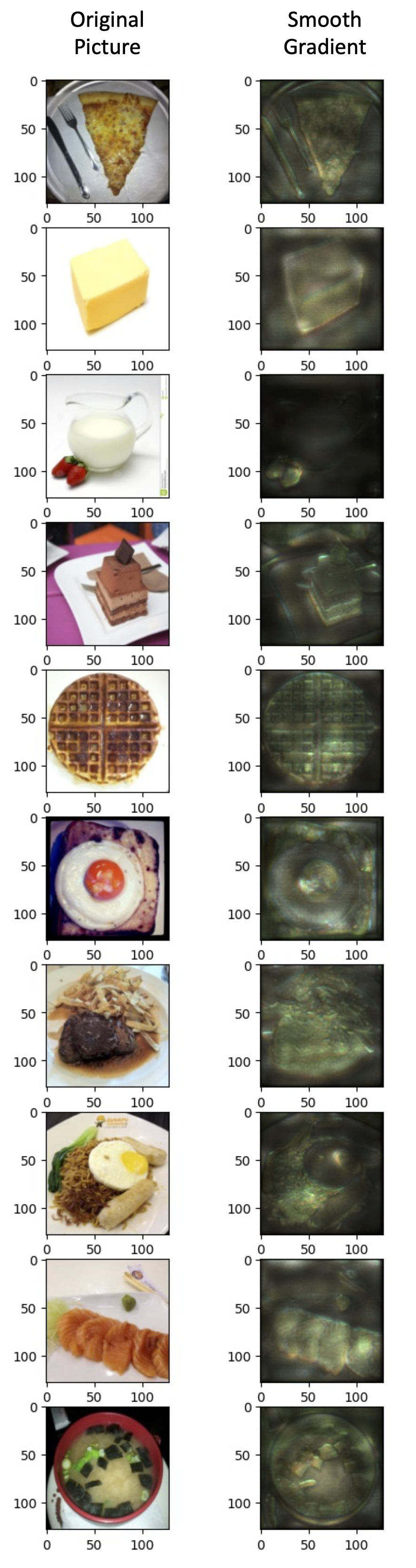
3.2. Smooth Gradient
An improvement of Saliency Map is Smooth Gradient Ref. Essentially, the method of Smooth Gradient is to randomly add noise to the image and get different heatmap, so the average of these heatmap would be more robust to noisy gradient.
# Smooth Gradient
def normalize(image):
  return (image - image.min()) / (image.max() - image.min())

def smooth_grad(x, y, model, epoch, param_sigma_multiplier):
  model_ft.eval()
  mean = 0
  sigma = param_sigma_multiplier / (torch.max(x) - torch.min(x)).item()
  smooth = np.zeros(x.cuda().unsqueeze(0).size())
  for i in range(epoch):
    noise = Variable(x.data.new(x.size()).normal_(mean, sigma**2)) # call Variable to generate random noise
    x_mod = (x+noise).unsqueeze(0).cuda()
    x_mod.requires_grad_()
    y_pred = model(x_mod)
    loss_func = torch.nn.CrossEntropyLoss()
    loss = loss_func(y_pred, y.cuda().unsqueeze(0))
    loss.backward()
    smooth += x_mod.grad.abs().detach().cpu().data.numpy() # similar to saliency map
  smooth = normalize(smooth / epoch) # normalization
  return smooth

smooth = []
for i, l in zip(images, labels):
  smooth.append(smooth_grad(i, l, model_ft, 500, 0.4))
smooth = np.stack(smooth)

fig, axs = plt.subplots(len(img_indices), 2, figsize=(5, 20))
for row, target in enumerate([images, smooth]):
  for column, img in enumerate(target):
    axs[column][row].imshow(np.transpose(img.reshape(3,128,128), (1,2,0)))
Similarly, the code blocks above shows the realization of Smooth Gradient, with the results shown below. Compared with results of Saliency Map shown in the previous section, we can see that both methods are able to show which pixels are critical for CNN model to understand the picture. In particular, Smooth Gradient method successfully reduces the noise and generates heatmap image with great detail.
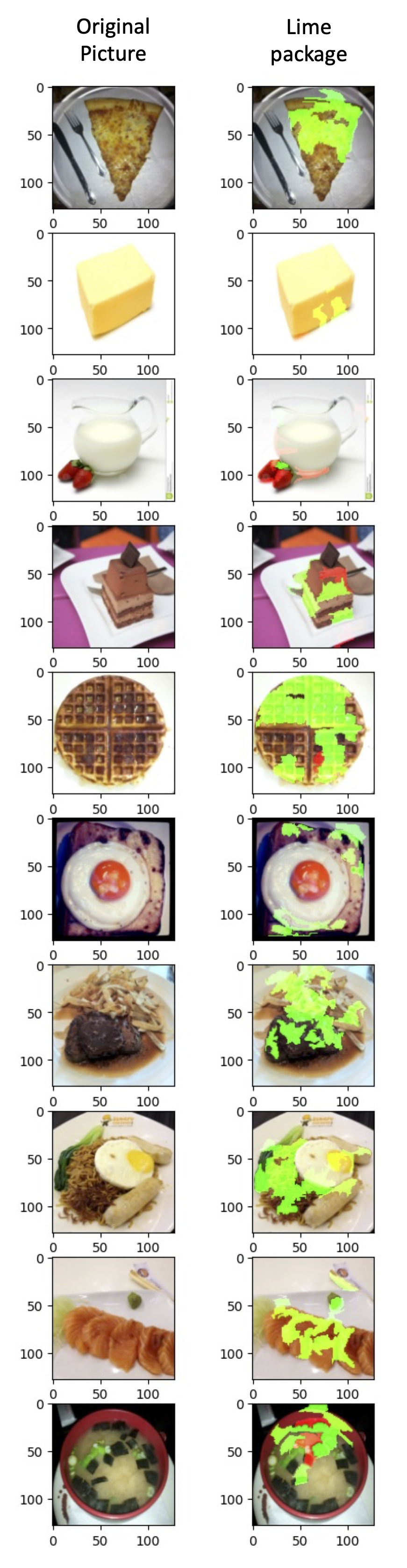
3.3. Local Interpretable Model-Agnostic Explanations (Lime)
Local Interpretable Model-Agnostic Explanations (Lime) is a popular package for CNN model visualization ref. In brief, it first splits the image into pieces with the help from skimage, and then performs locally weighted regression to get the explanation. The realization and results are shown below. Compare results of Lime with those from Smooth Gradient in the section above, I would prefer Smooth Gradient because it can provide much detailed explanations.
# Local Interpretable Model-Agnostic Explanations (Lime)
def predict(input):
    # input: numpy array, (batches, height, width, channels)
    model_ft.eval()
    input = torch.FloatTensor(input).permute(0, 3, 1, 2)
    # pytorch tensor, (batches, channels, height, width)
    output = model_ft(input.cuda())
    return output.detach().cpu().numpy()

def segmentation(input):
    return slic(input, n_segments=200, compactness=1, sigma=1, start_label=1)

fig, axs = plt.subplots(len(img_indices), 1, figsize=(4, 20))
np.random.seed(16)
for idx, (image, label) in enumerate(zip(images.permute(0, 2, 3, 1).numpy(), labels)):
    x = image.astype(np.double)
    explainer = lime_image.LimeImageExplainer()
    explaination = explainer.explain_instance(image=x, classifier_fn=predict, segmentation_fn=segmentation)
    lime_img, mask = explaination.get_image_and_mask(label=label.item(),positive_only=False,hide_rest=False,num_features=11,min_weight=0.05)
    axs[idx].imshow(lime_img)
plt.show()
plt.close()
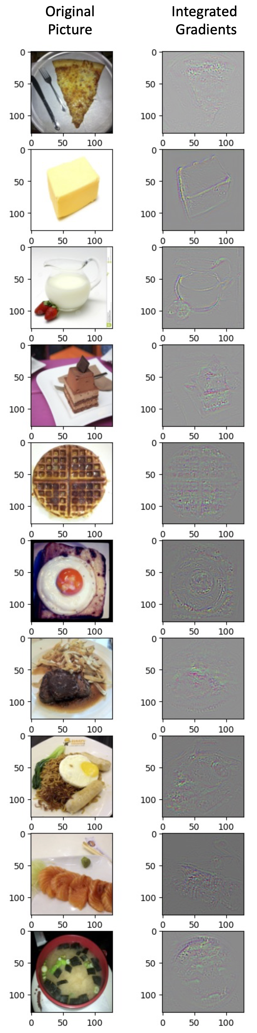
3.4. Integrated gradients
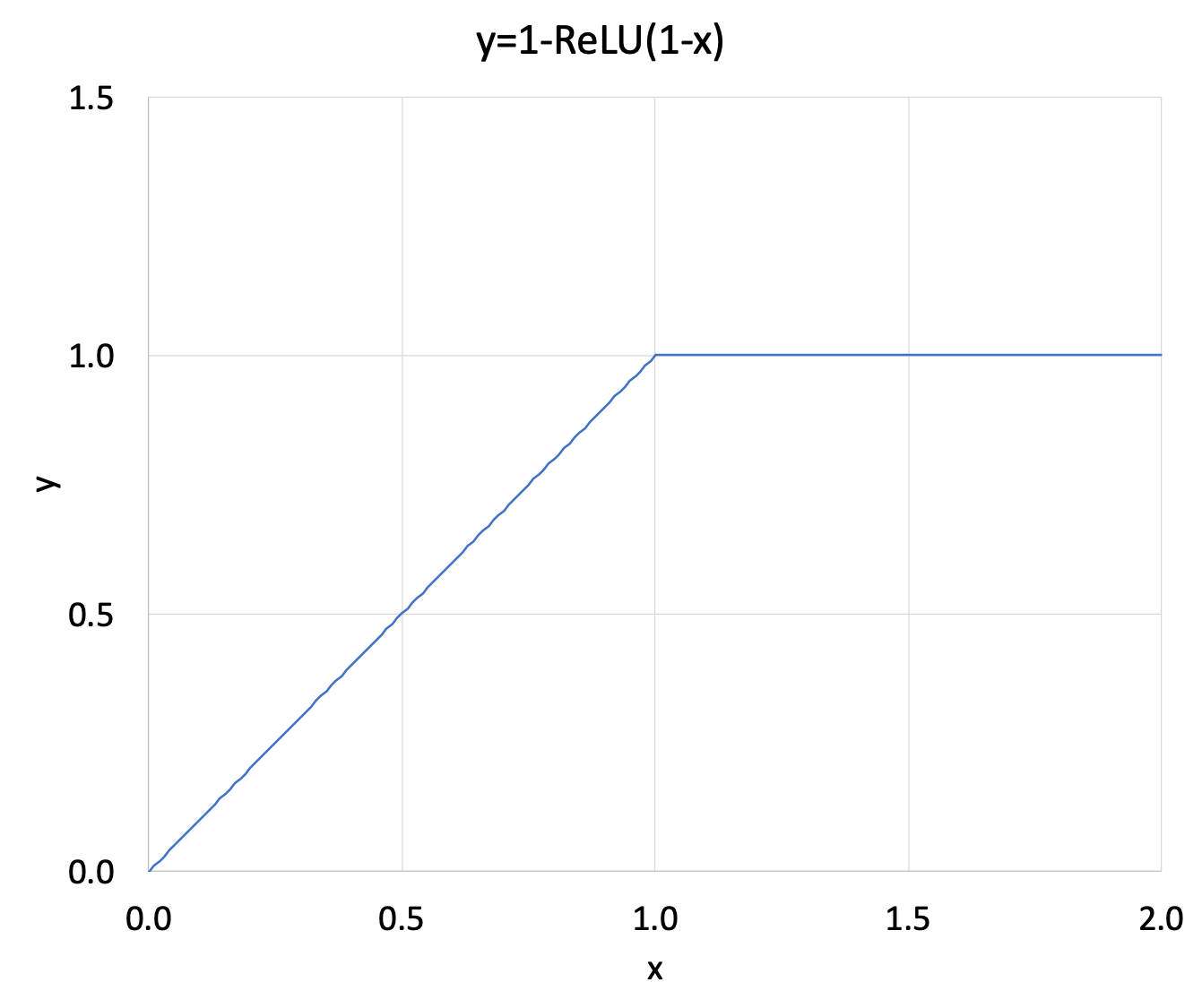
As pointed out by Sundararajan et al., one potential limitation of gradient based Explainable AI methods is the saturation of gradient (schematically illustrated by y=1-ReLU(1-x) function above). To resolve this potential issue, they developed Integrated gradients algorithm as shown by the equation below.

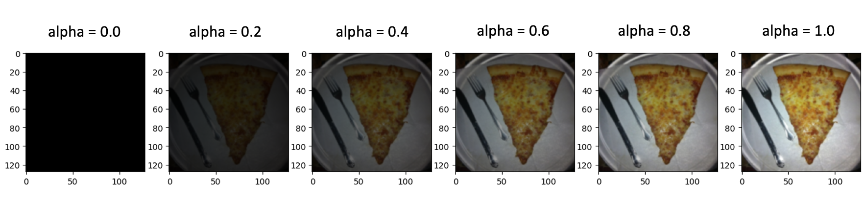
The picture below shows a five-step interpolation between the baseline x’ and the input image x for the first test image in this section. In the code block and the results below, we set interpolation step to 10.
# Integrated Gradients
class IntegratedGradients():
    def __init__(self, model):
        self.model = model
        self.gradients = None
        self.model.eval()

    def generate_images_on_linear_path(self, input_image, steps):
        xbar_list = [input_image*step/steps for step in range(steps+1)] # Generate scaled xbar images
        return xbar_list

    def generate_gradients(self, input_image, target_class):
        input_image.requires_grad=True # We want to get the gradients of the input image
        model_output = self.model(input_image) # Forward
        self.model.zero_grad() # Zero grads
        one_hot_output = torch.FloatTensor(1, model_output.size()[-1]).zero_().cuda() # Target for backprop
        one_hot_output[0][target_class] = 1
        model_output.backward(gradient=one_hot_output) # Backward
        self.gradients = input_image.grad
        gradients_as_arr = self.gradients.data.cpu().numpy()[0] # Convert Pytorch variable to numpy array
        return gradients_as_arr

    def generate_integrated_gradients(self, input_image, target_class, steps):
        xbar_list = self.generate_images_on_linear_path(input_image, steps) # Generate xbar images
        integrated_grads = np.zeros(input_image.size()) # Initialize an image composed of zeros
        for xbar_image in xbar_list:
            single_integrated_grad = self.generate_gradients(xbar_image, target_class) # Generate gradients from xbar images
            integrated_grads = integrated_grads + single_integrated_grad/steps # Add rescaled grads from xbar images
        return integrated_grads[0]

def normalize(image):
  return (image - image.min()) / (image.max() - image.min())

images, labels = train_set.getbatch(img_indices)
images = images.cuda()

IG = IntegratedGradients(model_ft)
integrated_grads = []
for i, img in enumerate(images):
  img = img.unsqueeze(0)
  integrated_grads.append(IG.generate_integrated_gradients(img, labels[i], 10))
fig, axs = plt.subplots(len(img_indices), 2, figsize=(5, 20))
for i, img in enumerate(images):
  axs[i][0].imshow(img.cpu().permute(1, 2, 0))
for i, img in enumerate(integrated_grads):
  axs[i][1].imshow(np.moveaxis(normalize(img),0,-1))
plt.show()
plt.close()
From this result, we can see that the method of Integrated gradients can indeed illustrate some very interesting patterns in the image. One particular strength of Integrated gradients is that this method is very easy to implement and can potentially handle various types of data.
4. Conclusions
In this project, I have developed a CNN based model for food image classification and achieved 99% accuracy on training set and 91% accuracy on test set. The bottom, mid, and top layers of model are then visualized by t-SNE technique. In addition, I have also employed four Explainable Artificial Intelligence techniques, including Saliency map, Smooth gradient, Lime package, and Integrated gradients, to better understand the model. Among these 4 techniques, I recommend Smooth gradient method, because it can effectively reduces noise and generates heatmap image with great detail.