Project 5: Using Autoencoder for Anomaly Detection and searching similar images
1. Overview
Anomaly detection is a technique used for identifying rare items, events or observations, which deviate significantly from the majority of the data and do not conform to a well defined notion of normal behavior wikipedia.
Anomaly detection has very wide applications, such as Fraud detection in credit card transactions ref, Network Intrusion detection ref, and Cancer cell detection ref.
A wide spectrum of techniques have been proposed for anomaly detection, some of the popular methods are: Density-based techniques (e.g., k-nearest neighbor), Cluster analysis-based techniques, Ensemble techniques, Long Short-Term Memory (LSTM) neural networks, as well as Autoencoders.
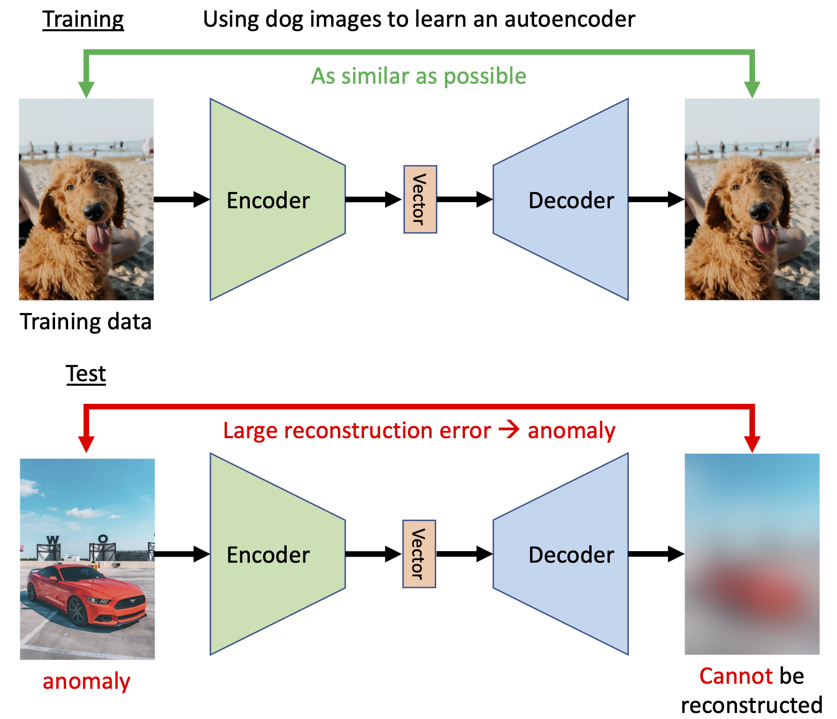
In this project, we will build an Autoencoder based anomaly detector, and we will use it to (1) determine whether the given image is similar to the training data (2) find images that are similar to the given image.
The Python Notebook containing the complete model development process and the data used in this project can be found at Google Drive.
2. Model development
2.1. Dataset
The dataset used in this project is the CIFAR-10 dataset from University of Toronto. This dataset consists of 60000 32x32 color images in 10 classes, with 6000 images per class. There are 50000 training images and 10000 test images. The 10 classes are: plane, car, bird, cat, deer, dog, frog, horse, ship, and truck.
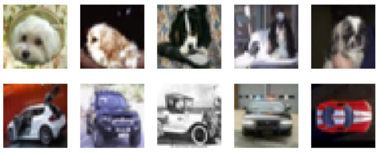
In this project, the training data contains 5000 images of dog from CIFAR-10 training images; the validation data contains 500 images of dog from CIFAR-10 test images; and the test data contains 500 images of dog and 500 images of car from CIFAR-10 test images. Sample images are shown below.
2.2. Methodology
Generally, the anomaly detector will be trained on a set of training data first. Then for a new input x, the anomaly detector will detect if x is similar to the training data. If answer is yes, then the new input x is considered normal. On the other hand, if the new input x is considered different from training data, then it will be considered anomaly (also known as outlier, novelty, or exceptions).
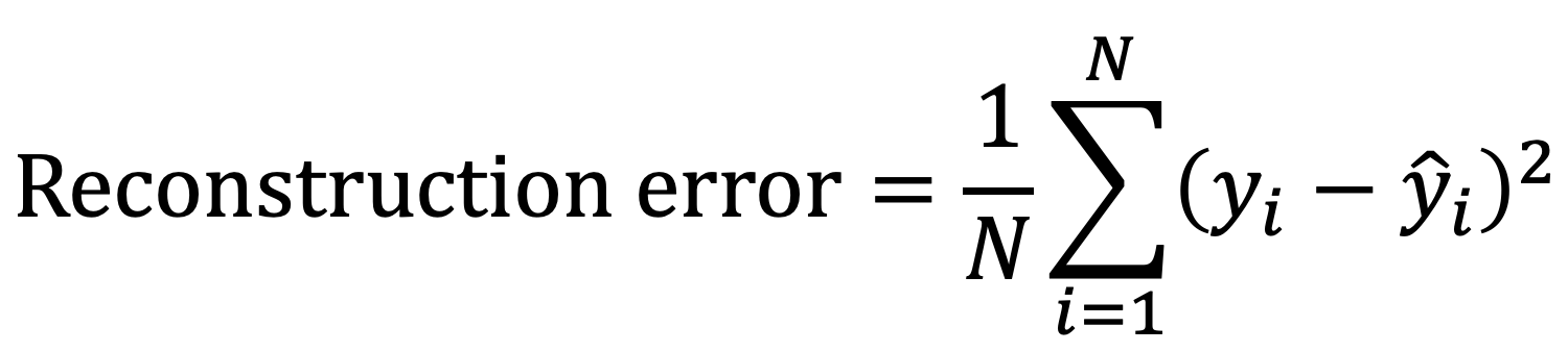
Specifically in our project, we will train an Autoencoder with small reconstruction error first. The definition and code realization of reconstruction error are shown below, followed by a figure demonstrating the effects of shifting and masking on reconstruction error.
def compare_imgs(img1, img2, title_prefix=""):
    # Calculate MSE loss between both images
    loss = F.mse_loss(img1, img2, reduction="sum")
    # Plot images for visual comparison
    grid = torchvision.utils.make_grid(torch.stack([img1, img2], dim=0), nrow=2, normalize=True, range=(-1,1))
    grid = grid.permute(1, 2, 0)
    plt.figure(figsize=(4,2))
    plt.title(f"{title_prefix} Loss: {loss.item():4.2f}")
    plt.imshow(grid)
    plt.axis('off')
    plt.show()

for i in range(2):
    # Load example image
    img = X_train[32 + 128* i]
    img = torch.from_numpy(img).float()
    img_mean = img.mean(dim=[1,2], keepdims=True)
    # Shift image by one pixel
    SHIFT = 1
    img_shifted = torch.roll(img, shifts=SHIFT, dims=1)
    img_shifted = torch.roll(img_shifted, shifts=SHIFT, dims=2)
    img_shifted[:,:1,:] = img_mean
    img_shifted[:,:,:1] = img_mean
    compare_imgs(img, img_shifted, "Shifted -")
    # Set half of the image to zero
    img_masked = img.clone()
    img_masked[:,:img_masked.shape[1]//2,:] = img_mean
    compare_imgs(img, img_masked, "Masked -")
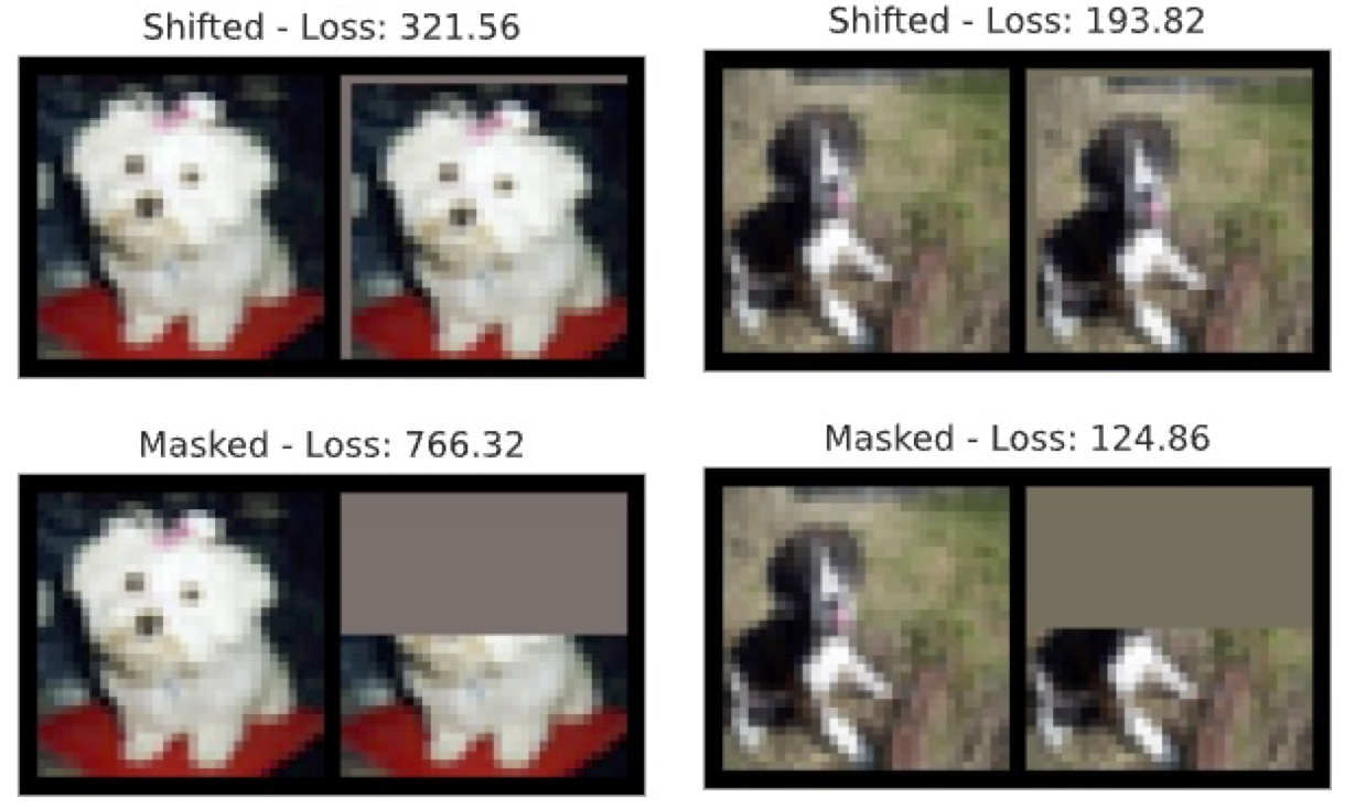
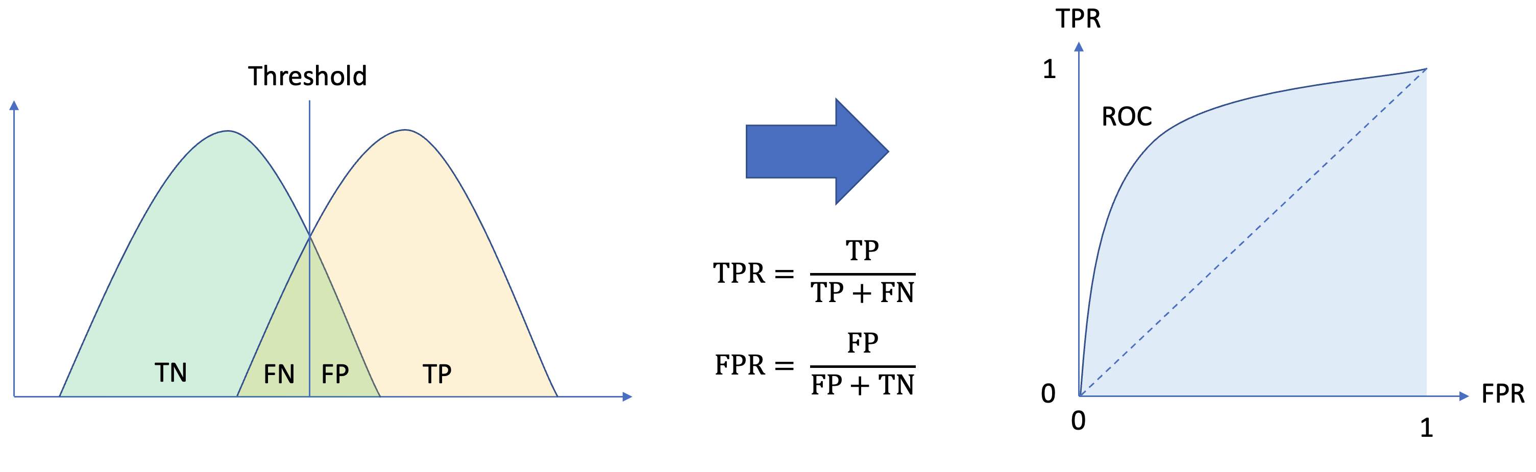
Then during the inference stage, we will use the reconstruction error as the anomaly score, as an image from an unseen distribution should have higher reconstruction error, and evaluate the performance of each model by its AUC (Area Under the Receiver operating characteristic (ROC) Curve) score.
2.3. Structure of Autoencoder model
A series of 12 autoencoder models are studied in this project. All of them share identical Encoder and Decoder, except the size of low dimensional bottleneck (also known as Latent, Embedding, Representation, and Code) Vector connecting them. The code block below shows the realization of an Autoencoder:
# Autoencoder models - Encoder
class Encoder(nn.Module):
    def __init__(self, num_input_channels : int, base_channel_size : int, latent_dim : int, act_fn : object = nn.GELU):
        super().__init__()
        c_hid = base_channel_size
        self.net = nn.Sequential(
            nn.Conv2d(num_input_channels, c_hid, kernel_size=3, padding=1, stride=2), # 32x32 => 16x16
            act_fn(),
            nn.Conv2d(c_hid, c_hid, kernel_size=3, padding=1),
            act_fn(),
            nn.Conv2d(c_hid, 2*c_hid, kernel_size=3, padding=1, stride=2), # 16x16 => 8x8
            act_fn(),
            nn.Conv2d(2*c_hid, 2*c_hid, kernel_size=3, padding=1),
            act_fn(),
            nn.Conv2d(2*c_hid, 2*c_hid, kernel_size=3, padding=1, stride=2), # 8x8 => 4x4
            act_fn(),
            nn.Flatten(),
            nn.Linear(2*16*c_hid, latent_dim))
    def forward(self, x):
        return self.net(x)

# Autoencoder models - Decoder
class Decoder(nn.Module):
    def __init__(self, num_input_channels : int, base_channel_size : int, latent_dim : int, act_fn : object = nn.GELU):
        super().__init__()
        c_hid = base_channel_size
        self.linear = nn.Sequential(
            nn.Linear(latent_dim, 2*16*c_hid),
            act_fn())
        self.net = nn.Sequential(
            nn.ConvTranspose2d(2*c_hid, 2*c_hid, kernel_size=3, output_padding=1, padding=1, stride=2), # 4x4 => 8x8
            act_fn(),
            nn.Conv2d(2*c_hid, 2*c_hid, kernel_size=3, padding=1),
            act_fn(),
            nn.ConvTranspose2d(2*c_hid, c_hid, kernel_size=3, output_padding=1, padding=1, stride=2), # 8x8 => 16x16
            act_fn(),
            nn.Conv2d(c_hid, c_hid, kernel_size=3, padding=1),
            act_fn(),
            nn.ConvTranspose2d(c_hid, num_input_channels, kernel_size=3, output_padding=1, padding=1, stride=2), # 16x16 => 32x32
            nn.Tanh()) # The input images is scaled between -1 and 1, hence the output has to be bounded as well
    def forward(self, x):
        x = self.linear(x)
        x = x.reshape(x.shape[0], -1, 4, 4)
        x = self.net(x)
        return x

class Autoencoder(pl.LightningModule):
    def __init__(self,base_channel_size: int,latent_dim: int,encoder_class : object = Encoder,decoder_class : object = Decoder,num_input_channels: int = 3,width: int = 32,height: int = 32):
        super().__init__()
        # Saving hyperparameters of autoencoder
        self.save_hyperparameters()
        # Creating encoder and decoder
        self.encoder = encoder_class(num_input_channels, base_channel_size, latent_dim)
        self.decoder = decoder_class(num_input_channels, base_channel_size, latent_dim)
        # Example input array needed for visualizing the graph of the network
        self.example_input_array = torch.zeros(2, num_input_channels, width, height)
    def forward(self, x):
        z = self.encoder(x)
        x_hat = self.decoder(z)
        return x_hat
    def _get_reconstruction_loss(self, batch):
        x = batch
        x_hat = self.forward(x)
        loss = F.mse_loss(x, x_hat, reduction="none")
        loss = loss.sum(dim=[1,2,3]).mean(dim=[0])
        return loss
    def configure_optimizers(self):
        optimizer = optim.Adam(self.parameters(), lr=1e-3)
        # Using a scheduler is optional but can be helpful.
        # The scheduler reduces the LR if the validation performance hasn't improved for the last N epochs
        scheduler = optim.lr_scheduler.ReduceLROnPlateau(optimizer, mode='min', factor=0.2, patience=20, min_lr=5e-5)
        return {"optimizer": optimizer, "lr_scheduler": scheduler, "monitor": "val_loss"}
    def training_step(self, batch, batch_idx):
        loss = self._get_reconstruction_loss(batch)
        self.log('train_loss', loss)
        return loss
    def validation_step(self, batch, batch_idx):
        loss = self._get_reconstruction_loss(batch)
        self.log('val_loss', loss)
    def test_step(self, batch, batch_idx):
        loss = self._get_reconstruction_loss(batch)
        self.log('test_loss', loss)
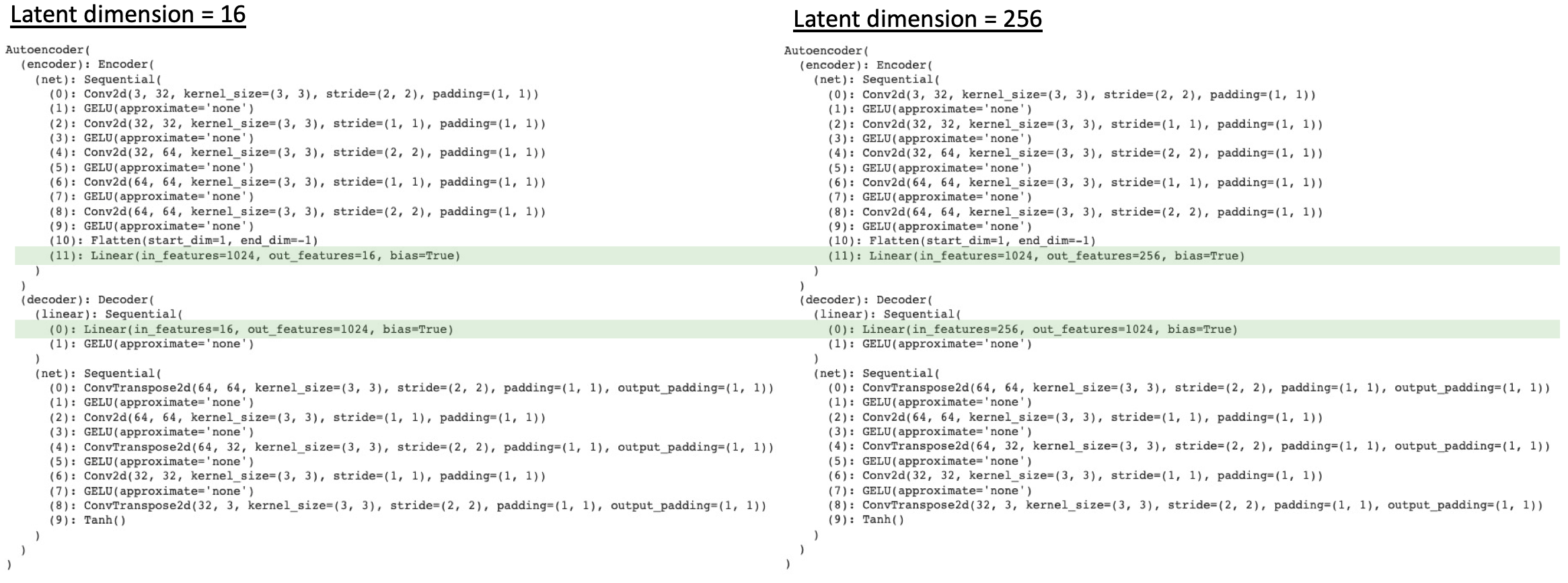
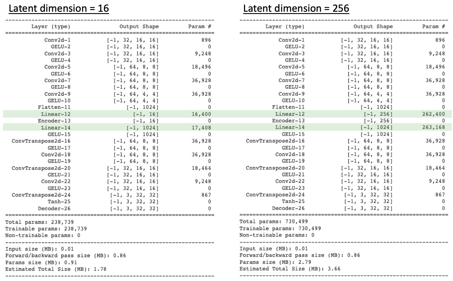
The figure below shows the summary of two autoencoders with latent dimension equals to 16 and 256. As can be seen from these figures, the only difference among various autoencoders is the size of latent vector. Also it is noticed that in order to accommodate the change in latent vector’s size, the last layer of Encoder and first layer of Decoder are modified too. As a consequence, the number of total parameters of each autoencoder is different too.
3. Results and discussion
3.1. Reconstruction error
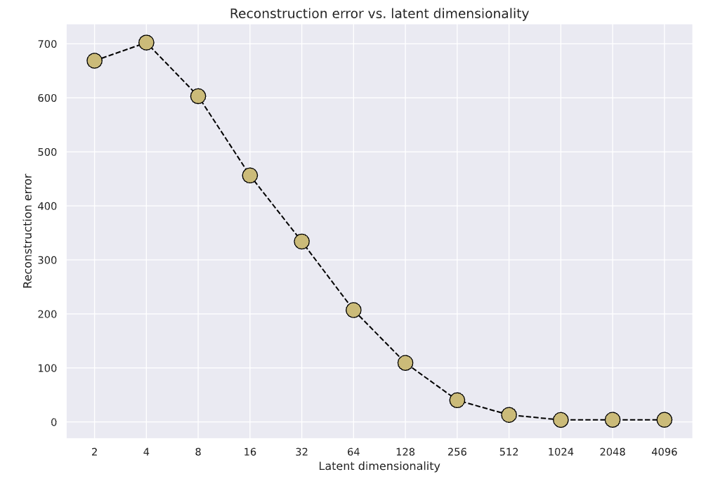
The figure below shows the result of reconstruction error as a function of latent vector dimension. From this figure, we can clearly observe the trend that, in general, as latent vector dimension increases, the reconstruction error will decrease significantly. This result is in good alignment with our expectation, because as the size of latent vector increases, less dimension reduction happened and more information is embedded in the latent vector. As a consequence, when Decoder tries to reconstruct the image using this larger latent vector, the reconstruction error will be lower.
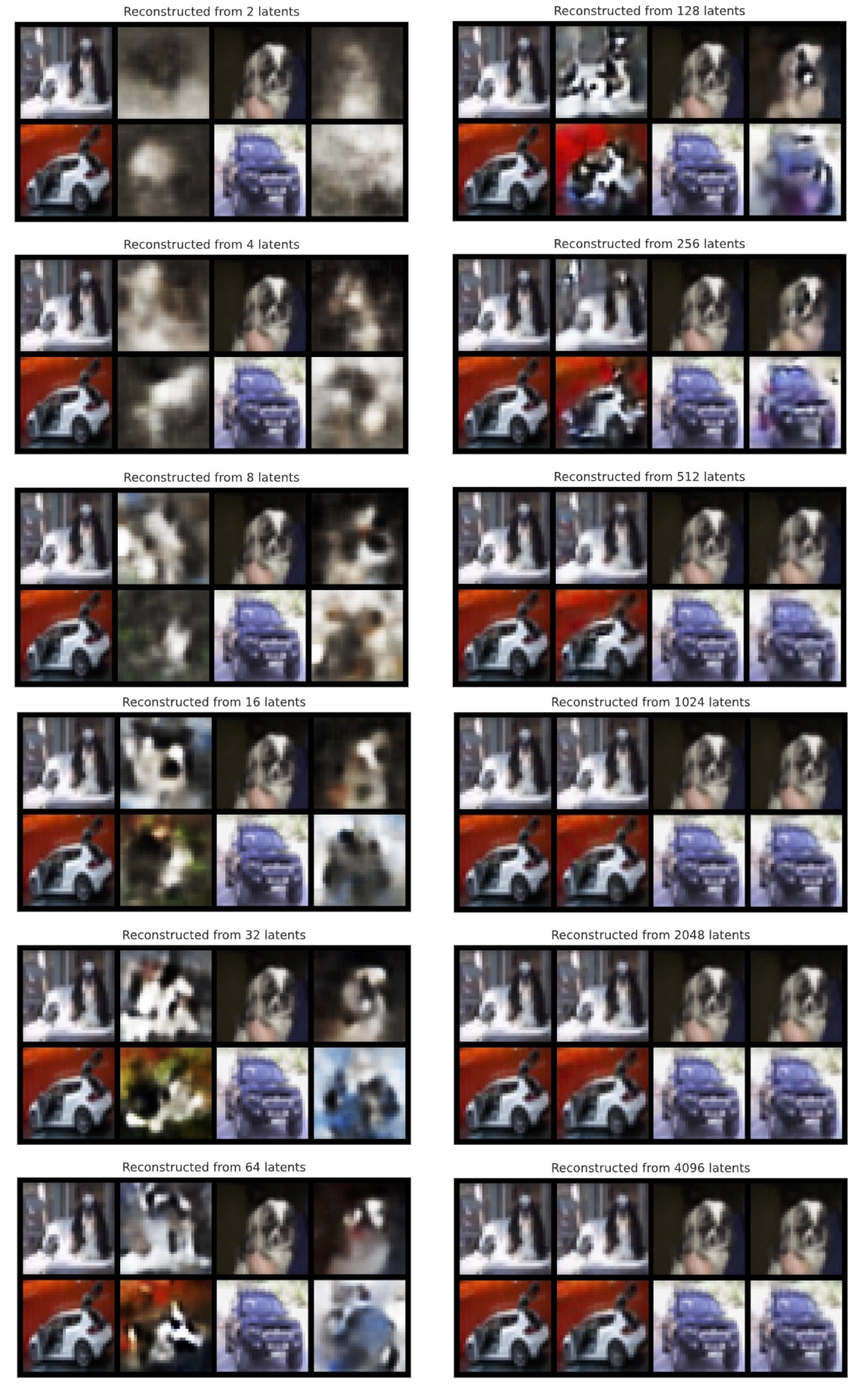
These pictures below shows the comparison of all 12 autoencoders with different latent vector. Two images from normal class (i.e., dog) and another two images from anomalous class (i.e., car) are employed. By taking a close look at these pictures, we can confirm that the quality of reconstructed images are indeed improved as we increase the size of the latent vector.
3.2. Area under the ROC curve (AUC)
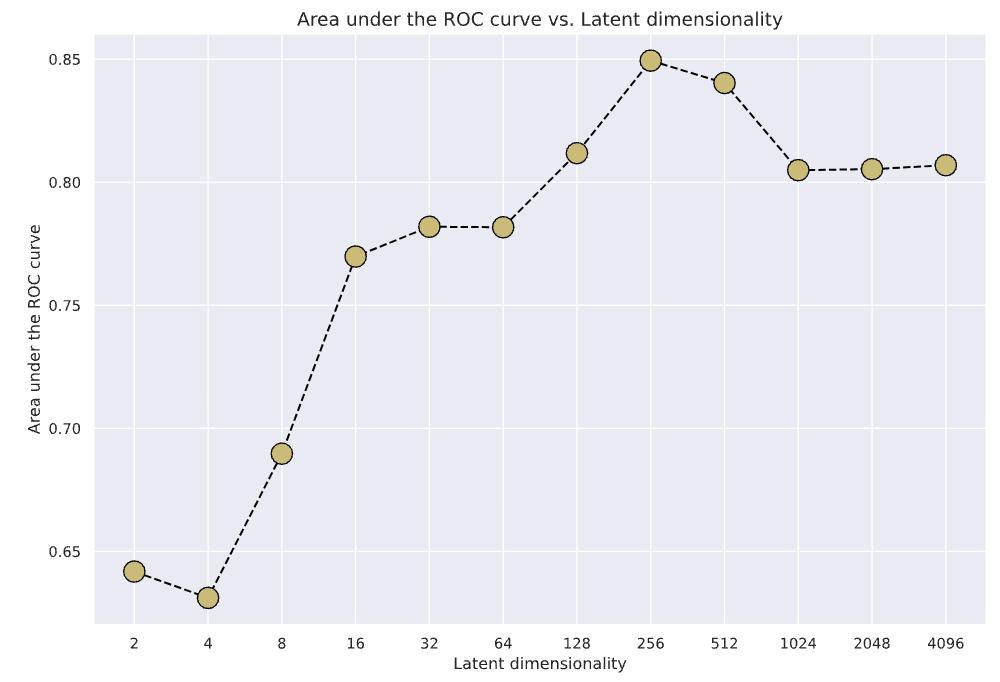
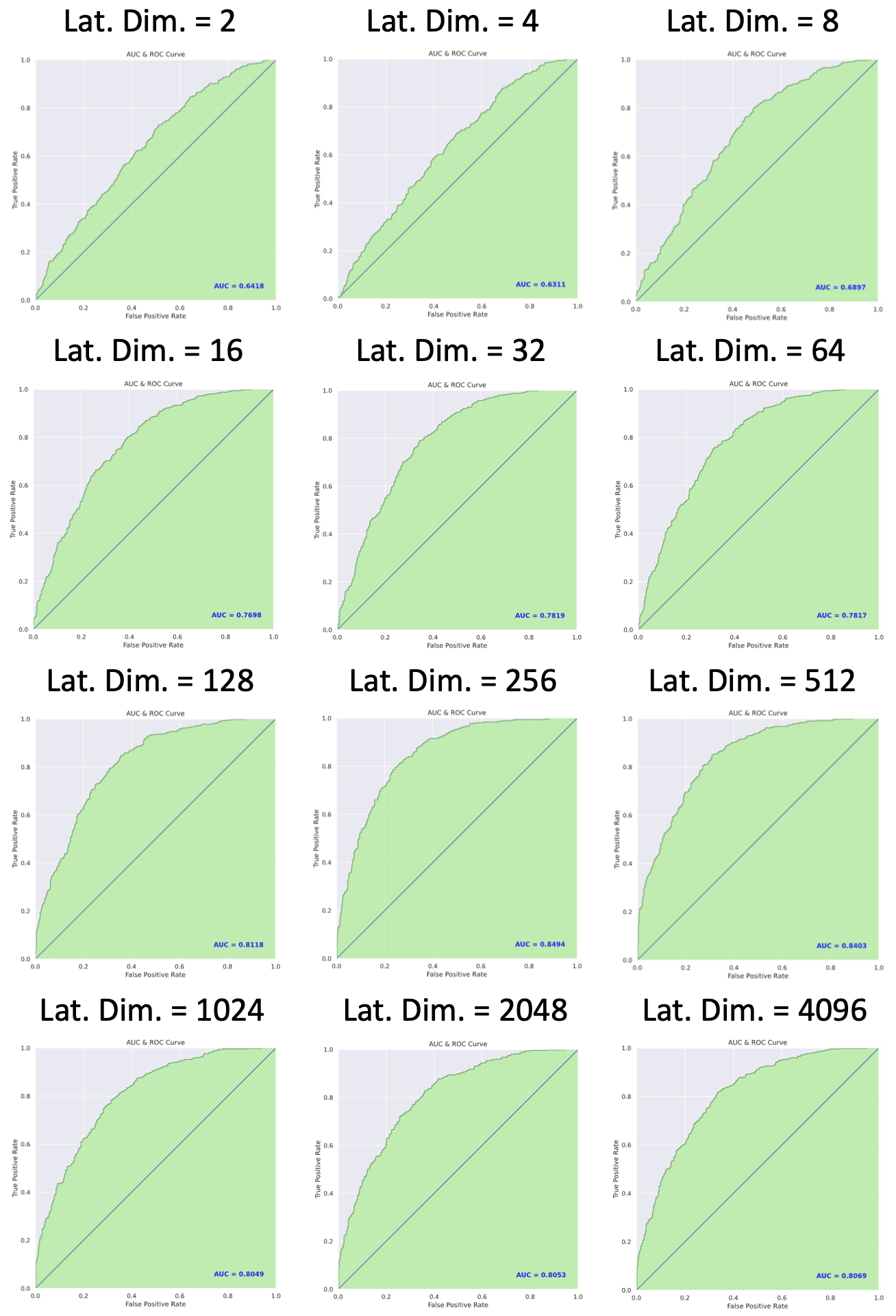
The figure below shows the summary of AUC scores of each model with different latent vector dimension, and the ROC curve of each model is shown in the next picture. From these figures, it is found that the highest AUC of 0.8494 occurred when latent vector dimension equals 256.
When the dimension of latent vector is very small (e.g., 2, 4, or 8), the AUC value is quite low. This is because as the latent vector is very small, very little information is embedded in the latent vector, both the normal image and anomalous image cannot be reconstructed well by the Decoder. As a consequence, both of them have large reconstruction errors, and the AUC score becomes quite low.
On the other hand, when the dimension of the latent vector is very high (1024, 2048, or 4096), the dimension of latent vector is so large and so much information is embedded in the latent vector that, both the normal image and anomalous image can be reconstructed very well. As a consequence, both of them have small reconstruction errors, and the AUC score becomes lower again. This trend can be observed in the figure above as well.
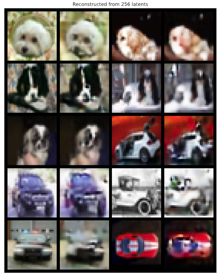
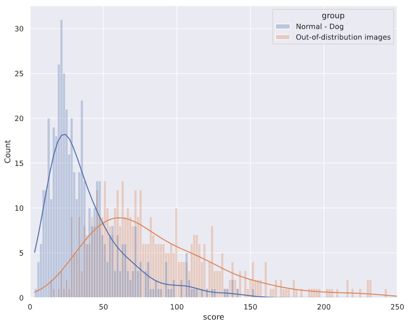
The figure below shows examples of original and reconstructed images of dog (normal) and car (anomalous) from Autoencoder with latent vector dimension equals 256. The next image shows the corresponding distribution of reconstruction error for normal and anomalous (aka out of distribution) images. From both images, we can see that the reconstructed images of dog indeed have better quality compared with those of car.
3.3. Out-of-distribution images
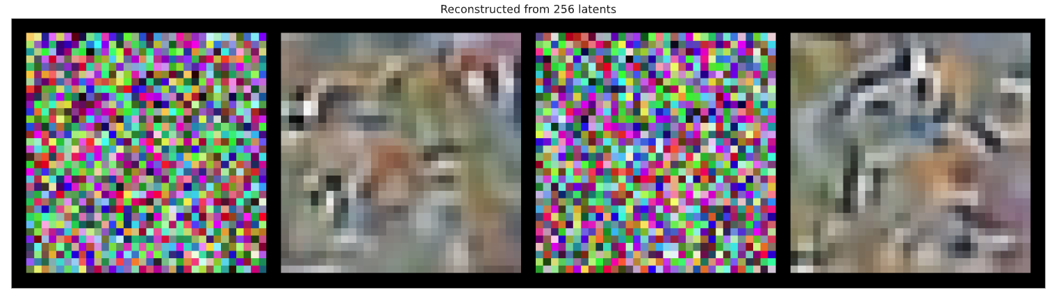
In this section, we will try to use Autoencoder to reconstruct images that are truly anomalous (i.e., out-of-distribution). The images below shows the comparison of original images and reconstructed images for (1) random images, (2) single color channel, (3) checkerboard pattern, and (4) color progression, with latent vector dimension set to 256. From these results, we can see that for these out-of-distribution images, even though very simple, their reconstructed images are of very low quality. This is great results for Autoencoder when used as an anomaly detector.

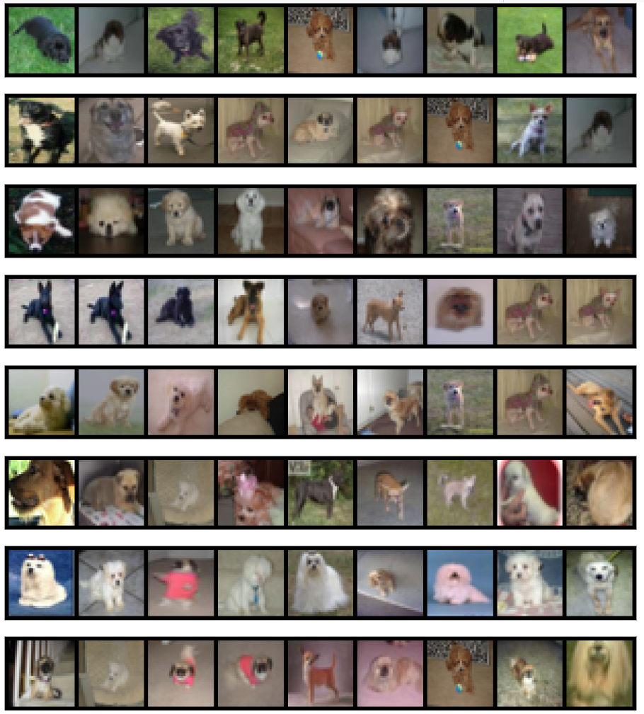
3.4. Searching similar images
Another application of Autoencoder is to find similar images of a given image. The figure below shows some very interesting results, and its code realization is shown in the following code block. As can be seen from these results, the Autoencoder we built in this project can successfully find images that are similar to a given image.
# Finding visually similar images
model = model_dict[256]["model"]

def embed_imgs(model, data_loader):
    # Encode all images in the data_loader using model, and return both images and encodings
    img_list, embed_list = [], []
    model.eval()
    for imgs in tqdm(data_loader, desc="Encoding images", leave=False):
        with torch.no_grad():
            z = model.encoder(imgs.to(model.device))
        img_list.append(imgs)
        embed_list.append(z)
    return (torch.cat(img_list, dim=0), torch.cat(embed_list, dim=0))

train_img_embeds = embed_imgs(model, train_loader)
test_img_embeds = embed_imgs(model, test_loader)

def find_similar_images(query_img, query_z, key_embeds, K=8):
    # Find closest K images. We use the euclidean distance here but other like cosine distance can also be used.
    dist = torch.cdist(query_z[None,:], key_embeds[1], p=2)
    dist = dist.squeeze(dim=0)
    dist, indices = torch.sort(dist)
    # Plot K closest images
    imgs_to_display = torch.cat([query_img[None], key_embeds[0][indices[:K]]], dim=0)
    grid = torchvision.utils.make_grid(imgs_to_display, nrow=K+1, normalize=True, range=(-1,1))
    grid = grid.permute(1, 2, 0)
    plt.figure(figsize=(12,3))
    plt.imshow(grid)
    plt.axis('off')
    plt.show()

# Plot the closest images for the first N test images as example
for i in range(8):
    find_similar_images(test_img_embeds[0][i], test_img_embeds[1][i], key_embeds=train_img_embeds)
4. Conclusions
In this project, I have developed a Autoencoder based model for anomaly detection that can successfully distinguish images of dog and car from CIFAR-10 dataset, with AUC equals to 0.8494. Furthermore, the Autoencoder model is also used to search for similar images of a given image, and very good results are obtained as well.