Project 6: Natural Language Inference with BERT and Explainable Artificial Intelligence

August 20, 2023

1. Overview

In this project, we will build a Bidirectional Encoder Representations from Transformers (BERT) based model for Natural Language Inference. The performance of the model will be evaluated on the Stanford Natural Language Inference (SNLI) Corpus. To further understand how it works, we will visualize attention mechanism and compare output embedding of BERT using Euclidean distance and Cosine similarity.

The Python Notebook containing the complete model development process and the data used in this project can be found at Google Drive.

2. Bidirectional Encoder Representations from Transformers (BERT)

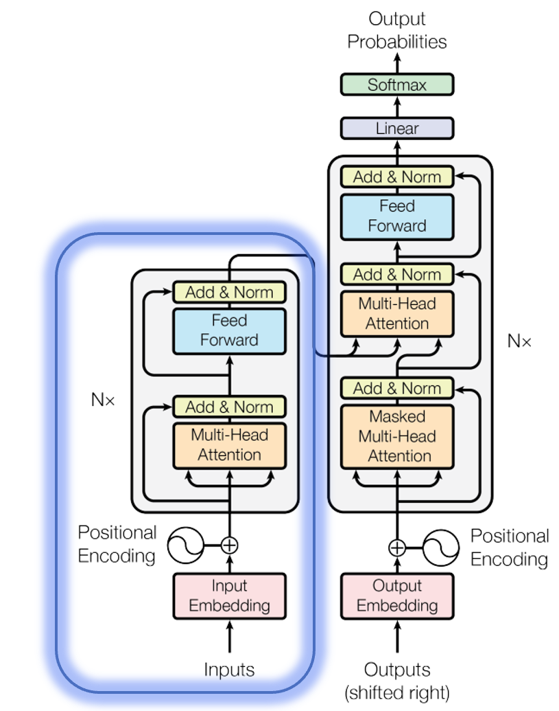
Bidirectional Encoder Representations from Transformers (BERT) arxiv is a language model developed by Google, based on the Encoder module of the Transformer model arxiv (see circled part of the figure below).

BERT has two variants (i.e., BERT_base and BERT_large), and their model architectures are summarized in the table below.

Model setting	BERT_base	BERT_large
Number of layers	12	24
Hidden size	768	1024
Number of self-attention heads	12	16
Total Parameters	110M	340M

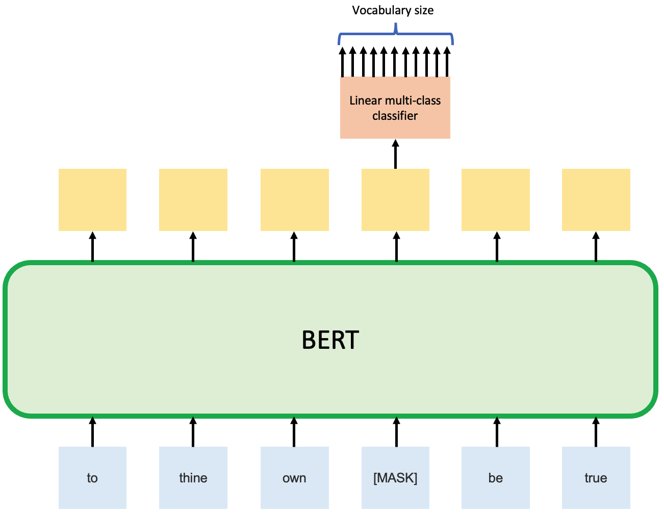
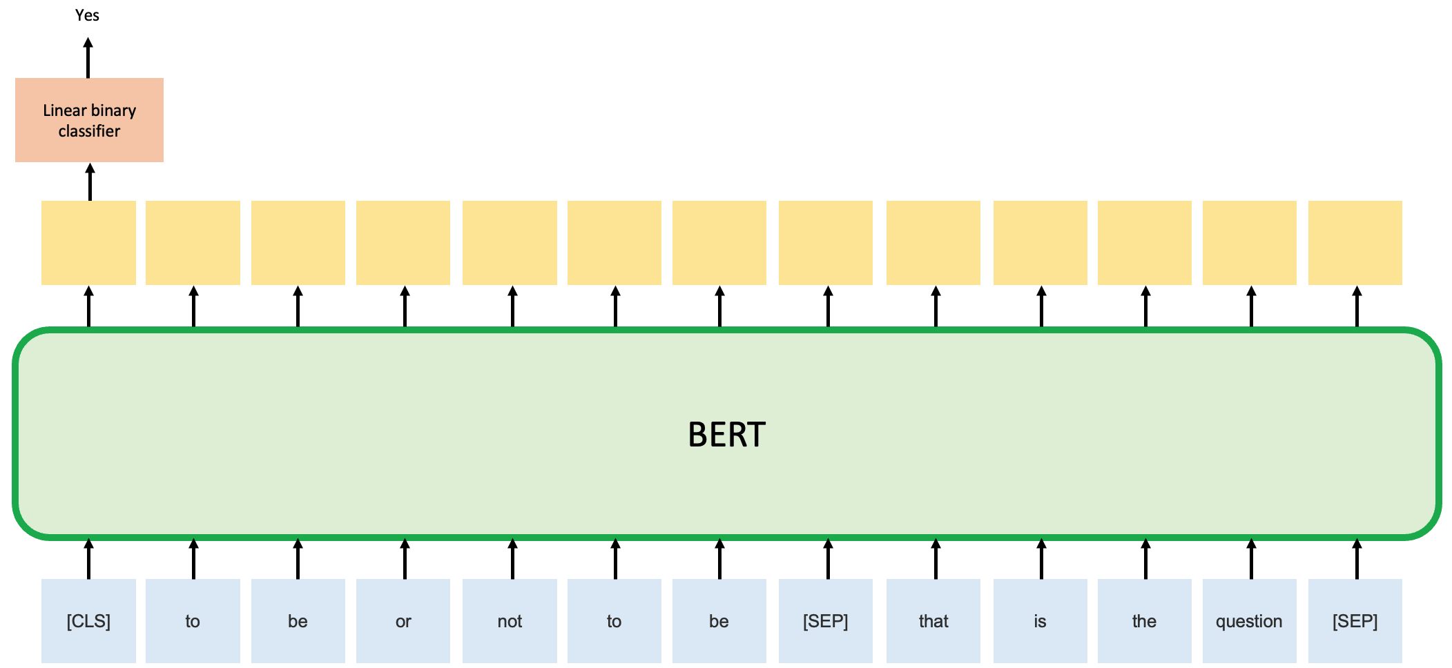
The BERT model is then pre-trained by two unsupervised tasks. Task 1 is Masked Language Model (Cloze task), which is predicting the masked word. Task 2 is Next Sentence Prediction (NSP), which is to predict whether sentence B is the actual next sentence that follow sentence A. The two figures below demonstrated these tasks schematically.

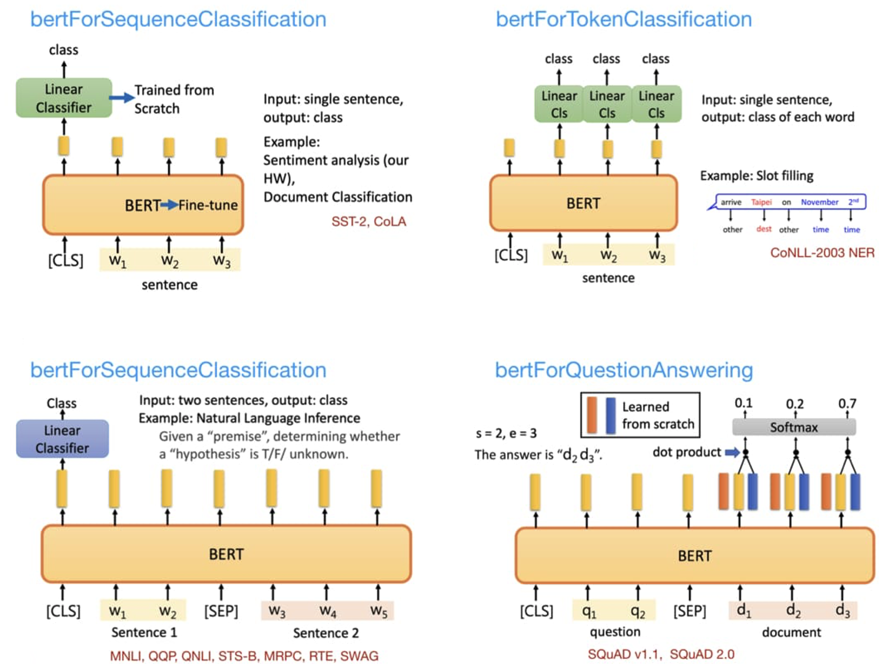
After pre-training, the BERT model can then be fine-tuned for various downstream tasks, as shown in the figure below source.

A range of BERT models are available on huggingface, such as:

bertModel
bertTokenizer
bertForMaskedLM
bertForNextSentencePrediction
bertForPreTraining
bertForSequenceClassification
bertForTokenClassification
bertForQuestionAnswering
bertForMultipleChoice

In this project, we will start with the baseline BERT model (i.e., bertModel) and build a Natural Language Inference model base on it manually. Because in this way, we can have a much deeper understanding of how BERT model actually works. In the next project (i.e., Question Answering), we will use a different approach and start from the bertForQuestionAnswering model instead.

3. Natural Language Inference (NLI)

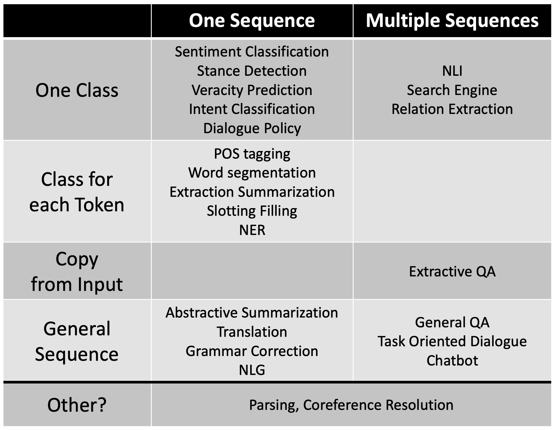
Natural Language Processing (NLP) is a broad topic. According to Professor Hung-yi Lee of National Taiwan University (NTU) website, a matrix can be developed by considering its input type (one sentence or multiple sentences) and output type (one class, class for each token, copy from input, or general sequence), as shown in the table below source.

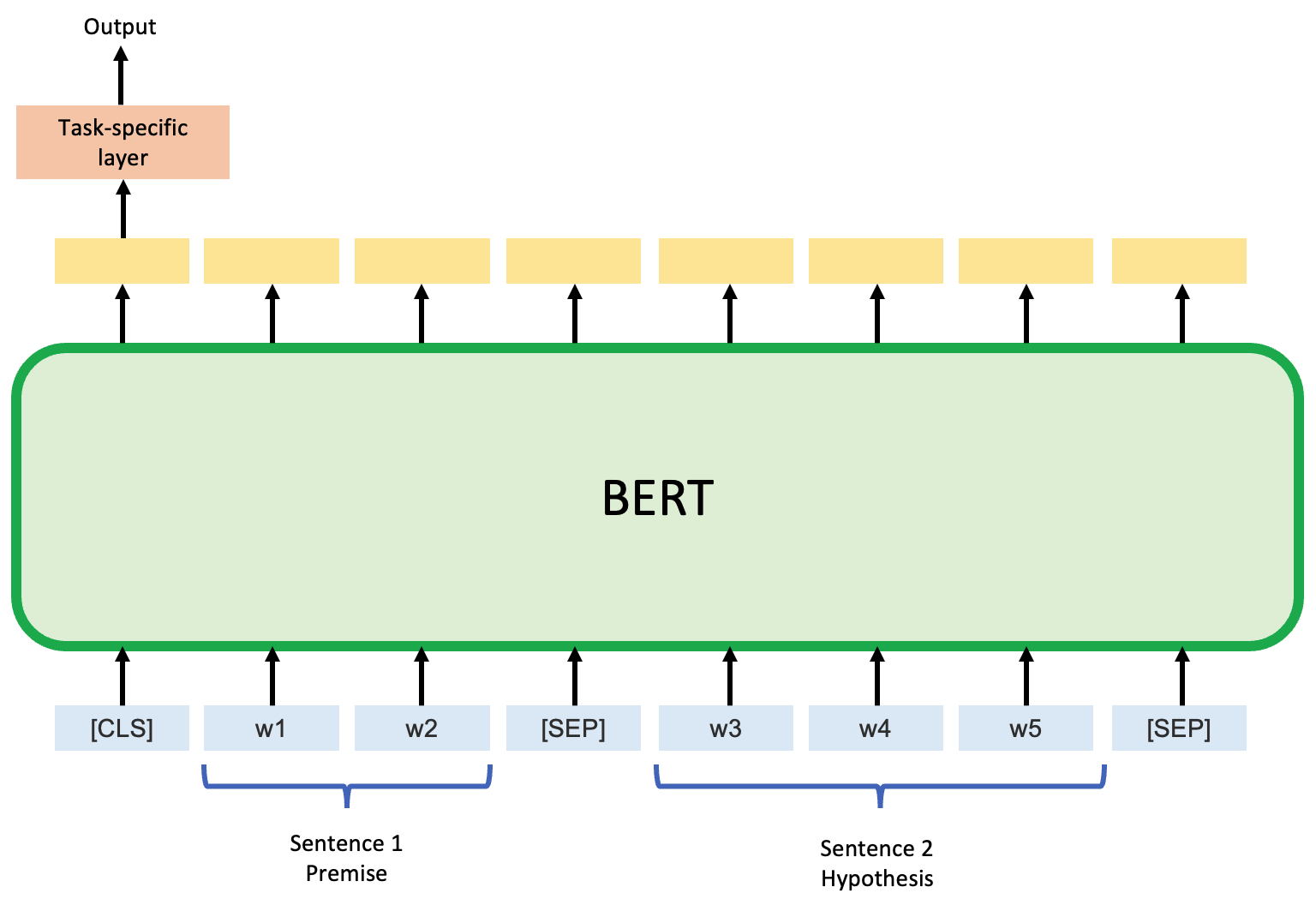
As shown in the figure below, for the Natural Language Inference (NLI) task that we are working on, it has two input sentences: one is premise, and the other is hypothesis Both sentences will be considered by BERT simultaneously. A task-specific layer will be added to the downstream of BERT for its first token (i.e., [CLS]), which will output the predicted relationship of these two sentences: entailment, contradiction, or neutral.

4. Model development

4.1. Data Pre-Processing

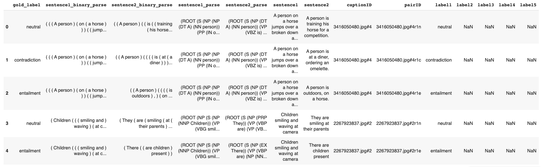
The Natural Language Inference (NLI) dataset we use is the Stanford Natural Language Inference (SNLI) Corpus. The SNLI corpus has 550,152 records in training set, 10,000 records in evaluation set and another 10,000 records in test set. The head of training set is shown below. Among all the columns, gold_label, sentence1, and sentence2 will be used, as they contain the inference results and the two sentences.

First we clean up the dataset by dropping records with incorrect gold_label. Only code for training set are shown below for brevity, similar procedures are also applied to the dev set and test set.

# removing the entries from all train, dev and test datasets with label '-'
df_train = df_train[df_train['gold_label'] != '-']
# dropping the rows from the data with NaN values
df_train = df_train.dropna(subset = ['sentence2'])
# analyzing the data
print(df_train.groupby('gold_label').count())
# Output
#                sentence1  sentence2
# gold_label                         
# contradiction     183185     183185
# entailment        183414     183414
# neutral           182762     182762

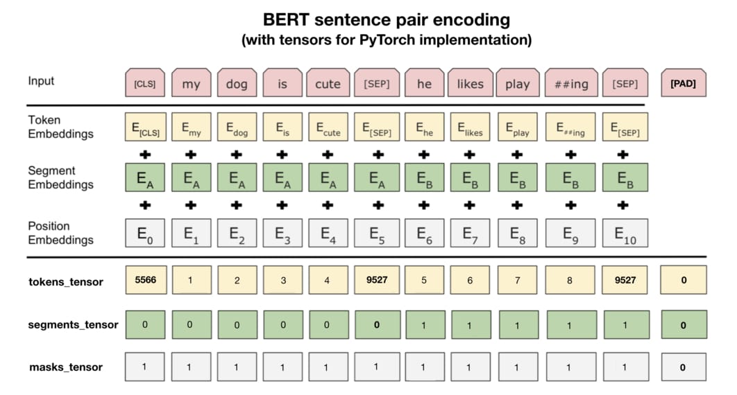
After the basic clean up, we need to further prepare the dataset so that it becomes compatible with BERT. The picture source below shows the required input for BERT. In particular, the Token Embeddings are the tokenized input sentences by wordpiece; the Segment Embeddings are used to identify whether the token is from the first sentence or the second sentence; and Position Embeddings are used to denote the position of each token.

In practice, when we use Pytorch BERT, we need to generate three tensors for the raw text data: tokens_tensor contains the id of each token; segments_tensor denotes the boundary of two sentences (0 for first sentence and 1 for second sentence); masks_tensor identifies the range of self-attention, as padding will be marked as 0 and no attention is needed in these locations.

First we will get the bert-base-uncased tokenizer and set the maximum sentence length to 128.

# using the same tokenizer used in pre-training
tokenizer = BertTokenizer.from_pretrained("bert-base-uncased")
# defining the maximum length of each sentence
max_sentence_length = 128

Then we will define some helper functions that we will use in the following steps.

# Tokenize Data by BertTokenizer
def tokenize_sentences(sentence):
  tokens = tokenizer.tokenize(sentence)
  return tokens

# Reduce the size of sentence to max_input_length
def reduce_sentence_length(sentence):
  tokens = sentence.strip().split(" ")
  tokens = tokens[:max_input_length]
  return tokens

# Trim the sentence to max_sentence_length
def trim_sentence(sentence):
  sentence = sentence.split()
  if len(sentence) >= max_sentence_length:
    sentence = sentence[:max_sentence_length]
  return " ".join(sentence)

# Get token type id of sentence 1
def token_type_ids_sent_01(sentence):
  try:
    return [0] * len(sentence)
  except:
    return []

# Get token type id of sentence 2
def token_type_ids_sent_02(sentence):
  try:
    return [1] * len(sentence)
  except:
    return []

# Get attention mask of given sentence
def attention_mask_sentence(sentence):
  try:
    return [1] * len(sentence)
  except:
    return []

# Convert the attention_mask and token_type ids to int
def convert_to_int(ids):
  ids = [int(d) for d in ids]
  return ids

# Combine the sequences from lists
def combine_sequence(sequence):
  return " ".join(sequence)

# Combine the masks
def combine_mask(mask):
  mask = [str(m) for m in mask]
  return " ".join(mask)

Next we will (1) trim the sentences to the maximum length, (2) add the [cls] and [sep] tokens, (3) apply the BertTokenizer to this newly generated sentences, (4) get the token type ids for the sentences, (5) obtain the sequence from the tokenized sentences, (6) generate attention mask, (7) combine the token type of both sentences, and finally (8) extract the required columns.

# trimming the sentences to the maximum length
df_train['sentence1'] = df_train['sentence1'].apply(trim_sentence)
df_train['sentence2'] = df_train['sentence2'].apply(trim_sentence)

# adding the [cls] and [sep] tokens
df_train['t_sentence1'] = cls_token + ' ' + df_train['sentence1'] + ' ' + sep_token + ' '
df_train['t_sentence2'] = df_train['sentence2'] + ' ' + sep_token

# applying the BertTokenizer to the newly generated sentences
df_train['b_sentence1'] = df_train['t_sentence1'].apply(tokenize_sentences)
df_train['b_sentence2'] = df_train['t_sentence2'].apply(tokenize_sentences)

# getting the token type ids for the sentences
df_train['sentence1_token_type'] = df_train['b_sentence1'].apply(token_type_ids_sent_01)
df_train['sentence2_token_type'] = df_train['b_sentence2'].apply(token_type_ids_sent_02)

# obtain the sequence from the tokenized sentences
df_train['sequence'] = df_train['b_sentence1'] + df_train['b_sentence2']

# generating attention mask
df_train['attention_mask'] = df_train['sequence'].apply(attention_mask_sentence)

# combining the token type of both sentences
df_train['token_type'] = df_train['sentence1_token_type'] + df_train['sentence2_token_type']

# Converting the inputs to sequential for torchtext Field
df_train['sequence'] = df_train['sequence'].apply(combine_sequence)
df_train['attention_mask'] = df_train['attention_mask'].apply(combine_mask)
df_train['token_type'] = df_train['token_type'].apply(combine_mask)

# extracting the required columns
df_train = df_train[['gold_label', 'sequence', 'attention_mask', 'token_type']]

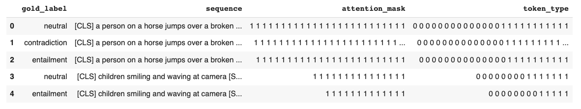
After these steps, the dataset will look like this (see figure below), and we finished 80% of data preprocessing.

# field for attention mask
ATTENTION = torchtext.data.Field(batch_first = True, use_vocab = False, tokenize = reduce_sentence_length, preprocessing = convert_to_int, pad_token = pad_token_idx)

# field for text
TEXT = torchtext.data.Field(batch_first = True, use_vocab = False, tokenize = reduce_sentence_length, preprocessing = tokenizer.convert_tokens_to_ids, pad_token = pad_token_idx, unk_token = unk_token_idx)

# text field for token type ids
TTYPE = torchtext.data.Field(batch_first = True, use_vocab = False, tokenize = reduce_sentence_length, preprocessing = convert_to_int, pad_token = 1)

# label field for label
LABEL = torchtext.data.LabelField()

fields = [('label', LABEL), ('sequence', TEXT), ('attention_mask', ATTENTION), ('token_type', TTYPE)]

train_data, valid_data, test_data = torchtext.data.TabularDataset.splits(path = 'snli_1.0_prep', train = 'snli_1.0_train_prep.csv', validation = 'snli_1.0_dev_prep.csv', test = 'snli_1.0_test_prep.csv', format = 'csv', fields = fields, skip_header = True)

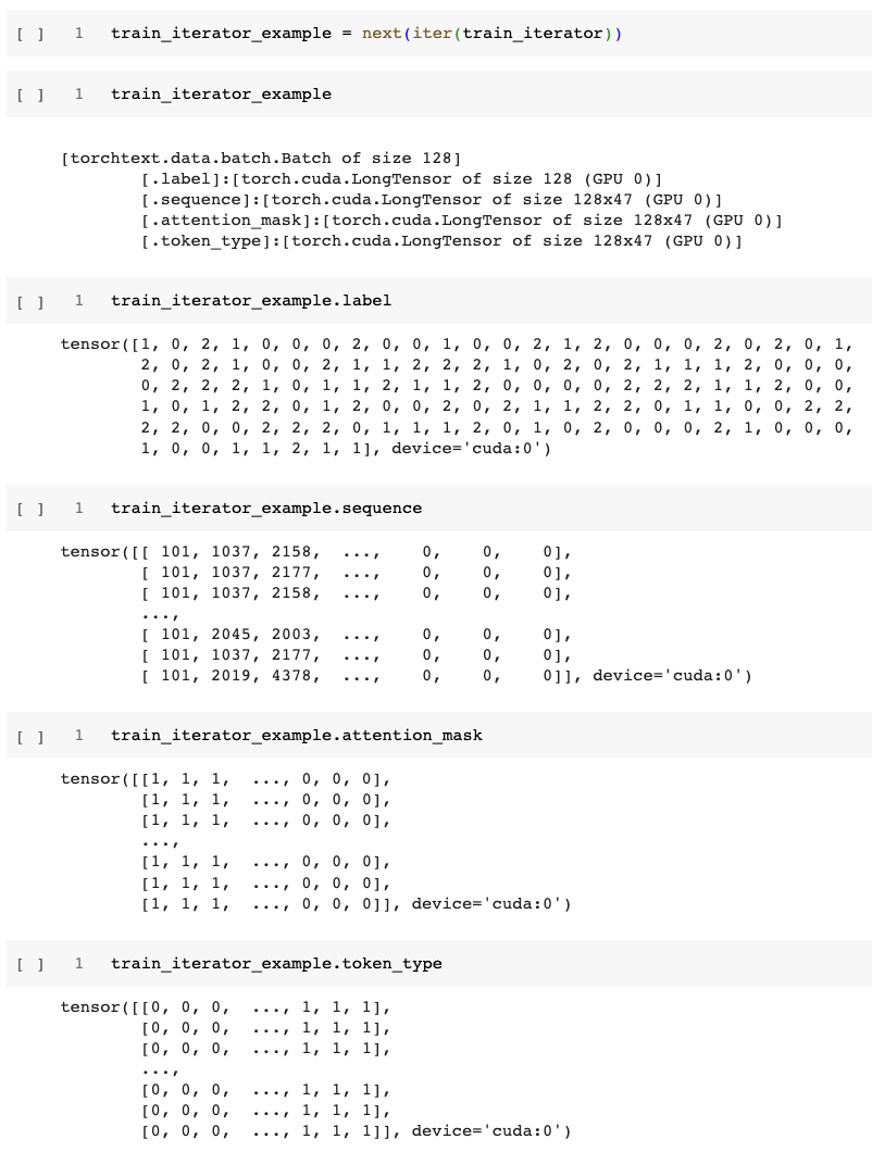
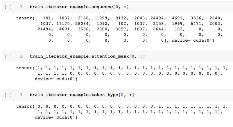
Then, with the help of the code block below, we will finish the data preprocessing and get the input data ready, as shown in the two figures below.

4.2. Model Training and Testing

# Model Training
# Using the pre-trained Bert_Model
bert_model = BertModel.from_pretrained('bert-base-uncased')

We start from the BERT base model as we discussed earlier. Then we will check the model configuration by model.config and we will get 'hidden_size': 768, as expected. Then as shown in the code block below, we add a task specific linear layer on top of the BERT base model. Since the NLI task has 3 outcomes (entailment, contradiction, neutral), the configuration of the top linear layer is 768 by 3.

class BERTNLIModel(nn.Module):
    def __init__(self, bert_model, output_dim,):
        super().__init__()
        self.bert = bert_model
        embedding_dim = bert_model.config.to_dict()['hidden_size']
        self.out = nn.Linear(embedding_dim, output_dim)

    def forward(self, sequence, attn_mask, token_type):
        embedded = self.bert(input_ids = sequence, attention_mask = attn_mask, token_type_ids = token_type)[1]
        output = self.out(embedded)
        return output

OUTPUT_DIM = len(LABEL.vocab)
model = BERTNLIModel(bert_model, OUTPUT_DIM,).to(device)

Then we create the training portion and testing potion of the model, define the optimizer, and train the model as shown below.

# Model Training
def train(model, iterator, optimizer, criterion, scheduler):
    print("Start Training ...")
    max_grad_norm = 1
    logging_step = 100
    epoch_loss = 0
    epoch_acc = 0
    model.train()
    step = 1
    train_loss = train_acc = 0

    # for batch in iterator:
    for batch in tqdm(iterator):
        optimizer.zero_grad() # clear gradients first
        torch.cuda.empty_cache() # releases all unoccupied cached memory
        sequence = batch.sequence
        attn_mask = batch.attention_mask
        token_type = batch.token_type
        label = batch.label
        predictions = model(sequence, attn_mask, token_type)
        loss = criterion(predictions, label)
        acc = accuracy(predictions, label)
        if fp16:
            accelerator.backward(loss)
        else:
            loss.backward()
        optimizer.step()
        scheduler.step()
        epoch_loss += loss.item()
        epoch_acc += acc.item()

        step += 1
        train_acc = train_acc + acc.item()
        train_loss = train_loss + loss.item()
        if step % logging_step == 0:
            print("learning_rate: ", optimizer.param_groups[0]["lr"])
            print(f"Epoch {epoch + 1} | Step {step} | loss = {train_loss / logging_step:.3f}, acc = {train_acc / logging_step:.3f}")
            train_loss = train_acc = 0
    return epoch_loss / len(iterator), epoch_acc / len(iterator)

# Model Testing
def evaluate(model, iterator, criterion):
    #print(iterator)
    epoch_loss = 0
    epoch_acc = 0
    model.eval()
    with torch.no_grad():
        # for batch in iterator:
        for batch in tqdm(iterator):
            sequence = batch.sequence
            attn_mask = batch.attention_mask
            token_type = batch.token_type
            labels = batch.label
            predictions = model(sequence, attn_mask, token_type)
            loss = criterion(predictions, labels)
            acc = accuracy(predictions, labels)
            epoch_loss += loss.item()
            epoch_acc += acc.item()
    return epoch_loss / len(iterator), epoch_acc / len(iterator)

# Defining the loss function and optimizer for our model
optimizer = AdamW(model.parameters(),lr=2e-5,eps=1e-6,correct_bias=False)
def get_scheduler(optimizer, warmup_steps):
    scheduler = transformers.get_constant_schedule_with_warmup(optimizer, num_warmup_steps=warmup_steps)
    return scheduler

# Prepare model
model, optimizer, train_iterator = accelerator.prepare(model, optimizer, train_iterator)
# model.load_state_dict(torch.load('P6-NLI.pt'))

N_EPOCHS = 20
warmup_percent = 0.2
total_steps = math.ceil(N_EPOCHS * train_data_len * 1./BATCH_SIZE)
warmup_steps = int(total_steps*warmup_percent)
scheduler = get_scheduler(optimizer, warmup_steps)

best_valid_loss = float('inf')

for epoch in range(N_EPOCHS):

    train_loss, train_acc = train(model, train_iterator, optimizer, criterion, scheduler)
    valid_loss, valid_acc = evaluate(model, valid_iterator, criterion)

    if valid_loss < best_valid_loss:
        best_valid_loss = valid_loss
        torch.save(model.state_dict(), 'P6-NLI-best.pt')

    print(f'\tTrain Loss: {train_loss:.3f} | Train Acc: {train_acc*100:.2f}%')
    print(f'\t Val. Loss: {valid_loss:.3f} |  Val. Acc: {valid_acc*100:.2f}%')

After training the model, we then evaluate the model’s performance on the test set, and we get pretty good accuracy of 87.83%.

model.load_state_dict(torch.load('P6-NLI.pt'))
test_loss, test_acc = evaluate(model, test_iterator, criterion)
print(f'Test Loss: {test_loss:.3f} |  Test Acc: {test_acc*100:.2f}%')
# Output
# Test Loss: 0.325 |  Test Acc: 87.83%

4.3. Results on custom inputs

One particle interesting thing to try is to provide two sentences by ourself and ask the NLI model we just built to predict the outcome on the fly. To achieve that goal, we need to add this block of code to our program.

# function to get the results on custom inputs
def predict_inference(premise, hypothesis, model, device):
    # appending the 'cls' and 'sep' tokens
    premise = cls_token + ' ' + premise + ' ' + sep_token
    hypothesis = hypothesis + ' ' + sep_token
    # tokenize the premise and hypothesis using bert tokenizer
    tokenize_premise = tokenize_sentences(premise)
    tokenize_hypothesis = tokenize_sentences(hypothesis)
    # generate the token type ids of both premise and hypothesis
    premise_token_type = token_type_ids_sent_01(tokenize_premise)
    hypothesis_token_type = token_type_ids_sent_02(tokenize_hypothesis)
    # combining the tokenized premise and hypothesis to generate the sequence
    indexes = tokenize_premise + tokenize_hypothesis
    # converting the sequence of tokens into token ids
    indexes = tokenizer.convert_tokens_to_ids(indexes)
    # combining the premise and hypothesis tokens ids
    indexes_type = premise_token_type + hypothesis_token_type
    # generating the attention mask of the ids
    attention_mask = token_type_ids_sent_02(indexes)
    # creating the pytorch tensors of indexes, indexes_type, attention_mask
    indexes = torch.LongTensor(indexes).unsqueeze(0).to(device)
    indexes_type = torch.LongTensor(indexes_type).unsqueeze(0).to(device)
    attention_mask = torch.LongTensor(attention_mask).unsqueeze(0).to(device)
    # predicting to get the judgements
    prediction = model(indexes, attention_mask, indexes_type)
    prediction = prediction.argmax(dim=-1).item()
    return LABEL.vocab.itos[prediction]

The following three blocks shows some representative results, and from them we can see that the model we build can indeed provide reasonable predictions as we expect.

premise = 'A black race car starts up in front of a crowd of people.'
hypothesis = 'A man is driving down a lonely road.'
predict_inference(premise, hypothesis, model, device)
# output
'contradiction'

premise = 'A soccer game with multiple males playing.'
hypothesis = 'Some men are playing a sport.'
predict_inference(premise, hypothesis, model, device)
# output
'entailment'

premise = 'A man playing an electric guitar on stage.'
hypothesis = 'A man is performing for cash'
predict_inference(premise, hypothesis, model, device)
# output
'neutral'

5. Understanding BERT model with Explainable AI techniques

5.1. Attention mechanism

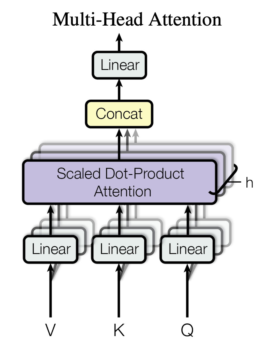
One of the key features in BERT is its multi-head attention mechanism, as shown in the figure below source.

To see how does attention mechanism actually work in our trained NLI model, we can utilize the BertViz module. The installation of BertViz module is shown below.

# Install BertViz
# Ref: https://colab.research.google.com/drive/1g2nhY9vZG-PLC3w3dcHGqwsHBAXnD9EY
import sys
!test -d bertviz_repo || git clone https://github.com/jessevig/bertviz bertviz_repo
if not 'bertviz_repo' in sys.path:
  sys.path += ['bertviz_repo']

# Import packages
from transformers import BertTokenizer, BertModel
from bertviz import head_view

# Display visualzation helper within jupyter notebook
def call_html():
  import IPython
  display(IPython.core.display.HTML('''
        <script src="/static/components/requirejs/require.js"></script>
        <script>
          requirejs.config({
            paths: {
              base: '/static/base',
              "d3": "https://cdnjs.cloudflare.com/ajax/libs/d3/3.5.8/d3.min",
              jquery: '//ajax.googleapis.com/ajax/libs/jquery/2.0.0/jquery.min',
            },
          });
        </script>
        '''))

Then we can provide two sentences and get the attention of each head on each layer.

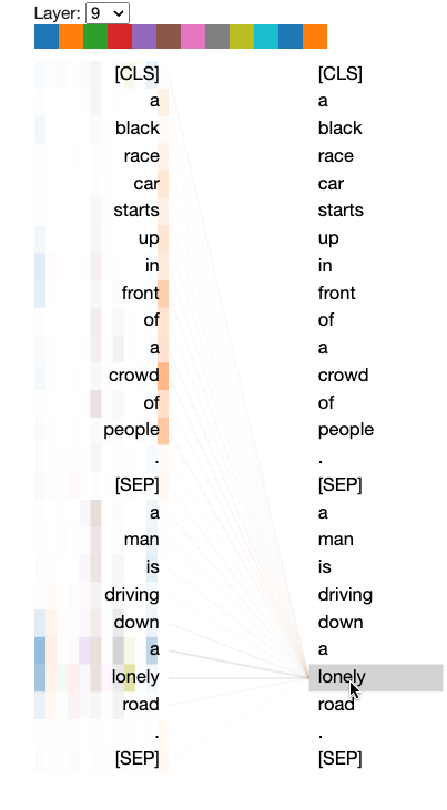
# two sentences
sentence_a = 'A black race car starts up in front of a crowd of people.'
sentence_b = 'A man is driving down a lonely road.'

# Display BERT attention
# Removing `state_dict` will get attention results of original BERT
model_version = 'bert-base-uncased'
finetuned_model  = BertModel.from_pretrained(model_version, output_attentions=True, state_dict=model.state_dict())

# Put tokens into BERT to get attention
inputs = tokenizer.encode_plus(sentence_a, sentence_b, return_tensors='pt', add_special_tokens=True)
token_type_ids = inputs['token_type_ids']
input_ids = inputs['input_ids']
attention = finetuned_model(input_ids, token_type_ids=token_type_ids)[-1]
input_id_list = input_ids[0].tolist() # Batch index 0
tokens = tokenizer.convert_ids_to_tokens(input_id_list)
call_html()
head_view(attention, tokens)

The attention of heads in layer 9 is shown below. As can be seen from the figure, the attention of lonely is heavily concentrated on a crowd of people and driving down a lonely road, which suggests that our BERT based NLI model detected the contradiction between these two sentences.

5.2. Contextualized word embeddings

Another very important feature of BERT is its contextualized word embeddings. To see how it works, we deliberately select 10 sentences with word duck:

Geese duck and teal are abundant
Hen and duck house
We enjoyed the subtle flavors of the duck
Apart from the duck and her two ducklings there is also a kangaroo and then a blue footed booby
Add the duck fat and bacon lardons and fry until golden brown
Do not duck your head down keep your shoulders hunched up and slowly stand up straight
I just need a place to duck out of the rain for a bit
The ceiling was so low I had to duck my head
If you hear gunfire duck and hide away from the windows
He slid up right behind her before she could duck into a shop

According to the Cambridge dictionary, duck as a noun refers to a bird that lives by water and has webbed feet, or the meat of this bird; duck, as a verb, means to move your head or the top part of your body quickly down, especially to avoid being hit, or to move quickly to a place, especially in order not to be seen. Sentences 1–5 has the first meaning of duck, and sentences 6–10 has the second meaning of duck.

# Index of word selected for embedding comparison. E.g. For sentence "Geese duck and teal are abundant", if index is 0, "Geese" is selected
select_word_index = [1, 2, 7, 3, 2, 2, 6, 8, 4, 9]

def euclidean_distance(a, b):
    # Compute euclidean distance (L2 norm) between two numpy vectors a and b
    dist = norm(a-b)
    return dist

def cosine_similarity(a, b):
    # Compute cosine similarity between two numpy vectors a and b
    cos_sim = dot(a, b)/(norm(a)*norm(b))
    return cos_sim

def get_select_embedding(output, tokenized_sentence, select_word_index):
    # The layer to visualize, choose from 0 to 12
    LAYER = 12
    # Get selected layer's hidden state
    hidden_state = output.hidden_states[LAYER][0]
    # Convert select_word_index in sentence to select_token_index in tokenized sentence
    select_token_index = tokenized_sentence.word_to_tokens(select_word_index).start
    # Return embedding of selected word
    return hidden_state[select_token_index].numpy()

# Metric for comparison. Choose from euclidean_distance, cosine_similarity
METRIC = euclidean_distance
# METRIC = cosine_similarity

# Tokenize and encode sentences into model's input format
tokenized_sentences = [tokenizer(sentence, return_tensors='pt') for sentence in sentences]

# Input encoded sentences into model and get outputs
with torch.no_grad():
    outputs = [model(**tokenized_sentence) for tokenized_sentence in tokenized_sentences]

# Get embedding of selected word(s) in sentences. "embeddings" has shape (len(sentences), 768), where 768 is the dimension of BERT's hidden state
embeddings = [get_select_embedding(outputs[i], tokenized_sentences[i], select_word_index[i]) for i in range(len(outputs))]

# Pairwse comparsion of sentences' embeddings using the metirc defined. "similarity_matrix" has shape [len(sentences), len(sentences)]
similarity_matrix = pairwise_distances(embeddings, metric=METRIC)

##### Plot the similarity matrix #####
plt.rcParams['figure.figsize'] = [12, 10] # Change figure size of the plot
# plt.imshow(similarity_matrix, cmap="jet", vmin=0, vmax=15) # Display an image in the plot
plt.imshow(similarity_matrix, vmin=6, vmax=16) # Display an image in the plot
# plt.imshow(similarity_matrix) # Display an image in the plot
plt.colorbar() # Add colorbar to the plot
plt.yticks(ticks=range(len(sentences)), labels=sentences) # Set tick locations and labels (sentences) of y-axis
plt.title('Comparison of BERT Word Embeddings') # Add title to the plot
for (i,j), label in np.ndenumerate(similarity_matrix): # np.ndenumerate is 2D version of enumerate
    plt.text(i, j, '{:.2f}'.format(label), ha='center', va='center') # Add values in similarity_matrix to the corresponding position in the plot
plt.show() # Show the plot

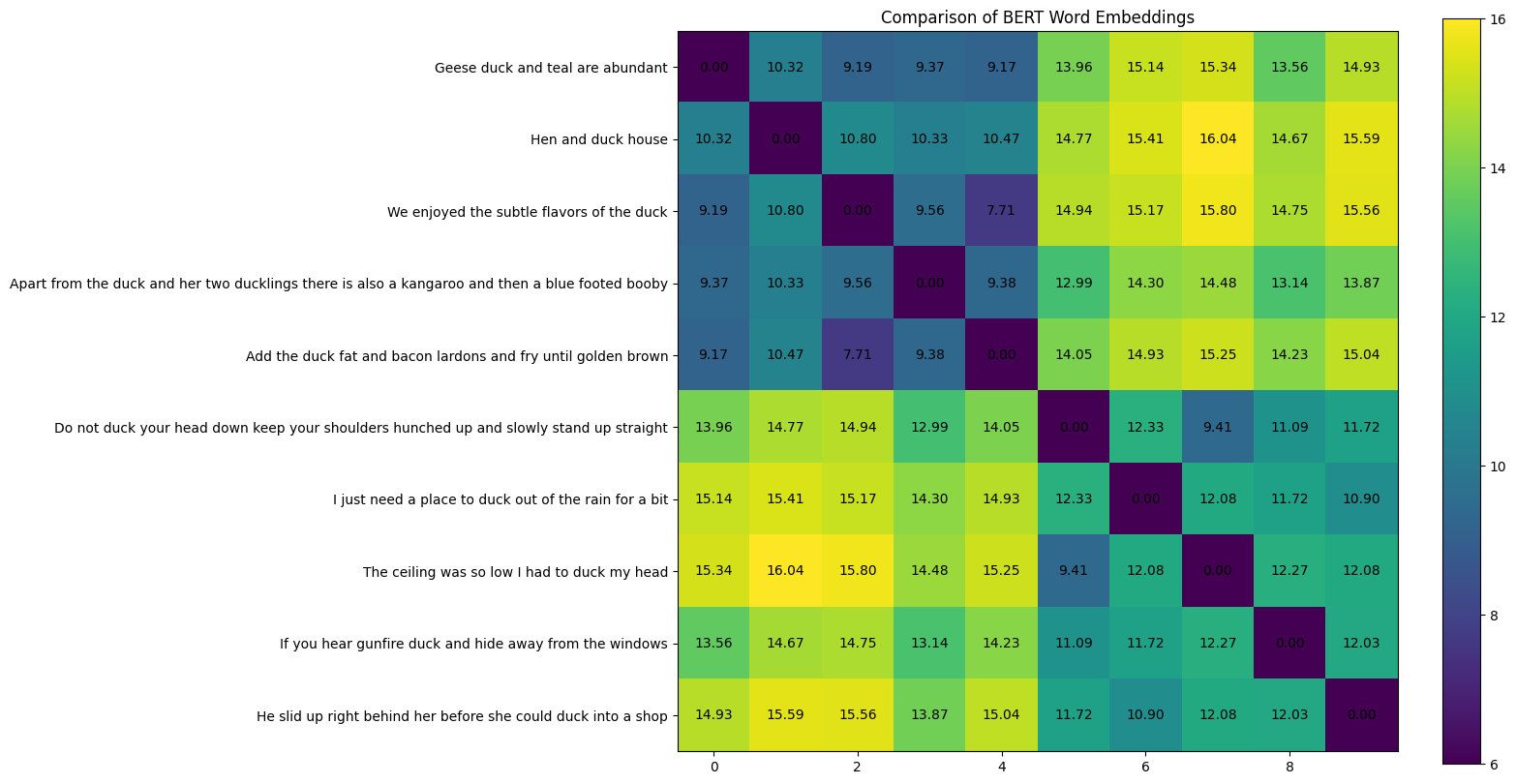
With the code block above, we compute the Euclidean Distance and Cosine Similarity of word duck for each sentence and shown in the two figures below. From the first figure, we can see that the first 5 sentences with duck as a noun has much smaller Euclidean Distance, similarly the other 5 sentences with duck as verb has smaller Euclidean Distance as well. The Euclidean Distances of sentences 1–5 and sentences 6–10 are much larger, as shown in the off diagonal parts clearly.

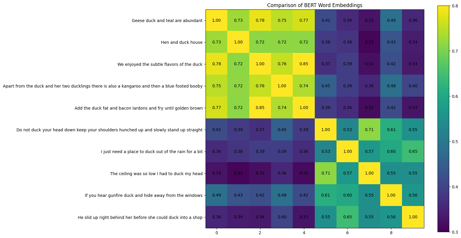
Similar trend can also be observed in the Cosine Similarity results shown below. Here, the first 5 sentences and the other 5 sentences have much larger Cosine Similarity among themselves, and the Cosine Similarity among them are much smaller. These results indicate that word embeddings in BERT are indeed contextualized and that different meanings of the same word can be distinguished successfully.

6. Conclusions

In this project, we built a BERT based Natural Language Inference model, and the model was fine-tuned on the Stanford Natural Language Inference (SNLI) Corpus with test accuracy equals to 87.83%. Then we visualized some key characteristics of the BERT model with Explainable AI techniques, including attention mechanism and contextualized word embeddings. Furthermore, we have also augmented the program so that it can provide predictions on custom inputs on-the-fly, and very good results are obtained as well.

References:

Source of hero image: https://medium.com/dissecting-bert/dissecting-bert-part2-335ff2ed9c73